Part I

You know, it all started when I was trying to visualize how the

Inverse Square Law (ISL)

would play out on a simple grid of whole integer numbers.

That led to the BIM (BBS-ISL Matrix) grid discovery.

Here is the simplified BIM with some new goodies!

Hint: The visual solution to the Goldbach Conjecture has never been simpler or more elegant!

Intro

The increasing squares 1–4–9–16–25… of the 1,2,3,4,5… numbers was well-established and could easily be visualized on a square matrix grid by placing the 1,2,3,4,5,… along each axis and making the central, primary or Prime Diagonal (PD) as the squares of those axial numbers -- giving the 1–4–9–16–25…

But what about all the other cells within the Inner Grid (IG)? What number values should be assigned to them?

Well, the 1^st Parallel Diagonal to the PD was found to be 3–5–7–9–11…, or simply the addition of 2 to the previous number (#). That 2 is simply 2 •1 or 2 times the Axis # 1 that starts that diagonal.

The 2^nd Parallel Diagonal was found to be 8–12–16–20–24…, or simply the addition of 4 to the previous #. That 4 is simply 2 •2, or 2 times the Axis # 2 that starts that diagonal.

The 3^rd Parallel Diagonal was found to be 15–21–27–33–39 or simply the addition of 6 to the previous #. That 6 is simply 2 •3, or 2 times the Axis # of 3 that start that diagonal.

See the pattern! Each Axis # • 2 equals the addition added to the previous # in that diagonal.

But how does one determine the first # on the diagonal in the IG? The short answer: take the PD value where the Row/Column intersects and subtract 1, e.i. 4–1=3, 9–1=8, 16–1=15.

Another method, one that really underscores how every IG # is determined, is to simply subtract the smaller from the larger PD value that intersects with ANY cell on the IG. Try it. It works for ANY and ALL IG cell # values, e.i., PD9-PD4=5, PD16-PD9=7, PD49-PD4=45, and so on.

So now we have a couple of ways to make the BIM -- any size BIM -- we want to work (and play) with!

TIPS

There are a couple of things that will make the BIM a whole lot easier to play with:

1. The BIM is symmetrical about the PD.
2. All the EVEN #s within the IG are ÷4. (The PD, too!)
3. All the ODD #s within the SIG (Strict Inner Grid = IG - 1^st Parallel Diagonal of 3–5–7–9–11 or all the ODD # ≥3) are NOT PRIMES.

The latter is the basis of the PRIMES vs NO-PRIMES. By subtracting any contiguous set of ODDs within the SIG from the corresponding 1^st Parallel Diagonal ODDS, one is left with just the PRIMES!

The number sequence 1–3–5–7–9… of ODDs is also known as the ODD Number Summation Series in that:

(0 + 1 = 1)

1 + 3 = 4

4 + 5 = 9

9 + 7 = 16

16 + 9 = 25 …

The 1--4--9--16--25--...? sequence is key to the entire BIM!

In other words, the Series itself generates the PD, the definitive Axis Squared Areas that define the essence of the ISL!

And, as No.2 above states, ALL the IG EVENS are ÷ 4, so what about 2–6–10–14–18–22–26–30… #s that are NOT ÷ 4?:

• Dividing them by 2 = 1–3–5–7–9–11–13–15…, respectively!

• Clearly, the ODD Number Summation Series helps define the BIM!

• Notice, too, that their differences are ÷4, in fact, equal 4.

• 2 + 6 = 8
• 6 + 10 = 16
• 10 + 14 = 24
• 14 + 18 = 32
• 18 + 22 = 40 …

• If you divide the sums by 8, you get 1, 2, 3, 4, 5…, respectively.

MathspeedST reveals some 200 of these "Rules" and more.

But let's move on.

The BIM is a 3-legged stool: ISL--PT--PRIMES

Pythagorean Triples

The Pythagorean -- Inverse Square Connection (TPISC I, II and III) were all about the Pythagorean Triples. You know, the non-isosceles, 90° right-triangles composed solely of natural Whole Integer Numbers (WINs).

If one simple drops down each PD Square # (≥9) until it intersects another Squared # on a BIM Row, one will have identified a Pythagorean Triple (PT) Row. Move along that Row and you will find another Squared #. These are the Squared sides of a PT, with the Squared longer-side hypotenuse at the PD intersection of that Row, e.i., drop the PD 9 down until it intersects the Squared # 16 on Row 5. There you will find the Squared # 9 and at the PD intersect, the Squared # 25, as 3² + 4² = 5².

It turns out that the PTs ONLY fall on Rows ÷24. (Rows ÷ 24 are Rows whose 1^st cell # is divisible by 24.)

PRIMES

It also turns out that those stealthily hidden PRIMES also ONLY fall on these Rows ÷24. Sometimes they match PTs, other times they don't, sometimes only one but not the other, and sometimes neither.

The real secret of the PRIMES on the BIM (POB), is that their pattern is revealed when they come as symmetrical pairs -- PRIME Pairs (PP) sets. Every EVEN # can be shown to be composed of 2 PRIMES -- PPsets -- that are positioned symmetrical on the BIM Axis to either side of a given EVEN #. In many cases, there are two or more PPsets that can form said EVEN #.

Running a diagonal perpendicular to the PD such that it runs from an EVEN # on the Upper Horizontal Axis to the Lower Vertical Axis, will intersect each and every PPset that forms -- i.e., the sums of the PPset equals the EVEN # -- that EVEN. And the number of STEPS to each PPset will identify the exact location of each PPset in its symmetrical location on the Axis! It's like magic! The PRIMES, when treated as PPsets, reveal a simple, easily visualized pattern of symmetry and fractal-like groupings across & down the entire BIM. In doing so, they provide a complete proof of Euler's Strong Form of the Goldbach Conjecture: every EVEN (≥2) is composed of two PRIMES.

Let's state that more explicitly:

On the BIM, Axis to Axis DIAGONALS between the same EVEN # always intersect one or more PRIME Pair sets (PPsets), the sum(s) of which equals said EVEN. The members of each PPset are located a symmetrically-even number of steps to either side of the said EVEN/2 on the Axis. Additionally, the STEPS along the DIAGONAL -- starting from either Axis -- to each PPset correspond to their location on the Axis. This, along with the Periodic Table Of PRIMES (PTOP), proves Euler's Strong Form of the Goldbach Conjecture.

Now let's break this down with a clear visual example: EVEN # = 10.

1. Draw a DIAGONAL between the 10's found on each Axis.
2. Note that there are 10 STEPS from one Axis to the other.
3. Halfway, at STEP 5, the DIAGONAL intersects the PD at 25.
4. This PD 25 is the Square of 5 as 5•5, and 5,5 = PPset, as 5+5=10.
5. At STEP 3 along the DIAGONAL, the intersect = 3,7 PPset, i.e., that BIM cell is located at the intersect of Column 7, Row 3, and 3+7=10.
6. At STEP 7 along the DIAGONAL, the intersect = 3,7 PPset, i.e., that BIM cell is located at the intersect of Column 3, Row 7, and 7+3=10
7. Note the symmetry in no.5 and 6 above. On either side of the PD, there will always be a mirror-symmetrical PPset. By convention, the PPsets are listed with the smaller # first.
8. At the halfway PD 25, draw a vertical line up to the top Axis at 5 = 10/2.
9. Locate the Axis 3 and Axis 7 numbers, noting that they are 3 STEPS and 7 STEPS from the origin 0, and, that they are symmetrically located to either side of the Axis 5, that, in this case, happens to also be a PPset of 5,5.
10. ALL EVENS will follow this same PRIMES On the BIM (POB) pattern.

Let's repeat this example with images!

Animated Gif Overview. Vimeo video is found just before the Summary.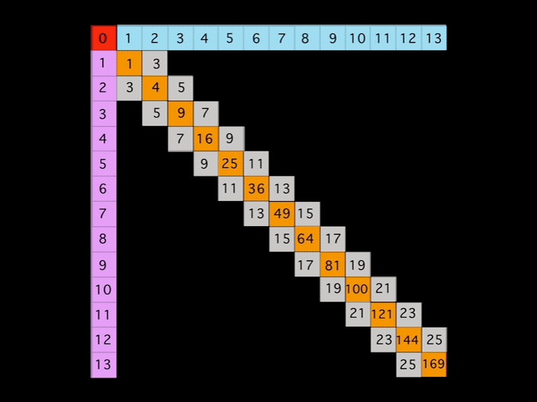

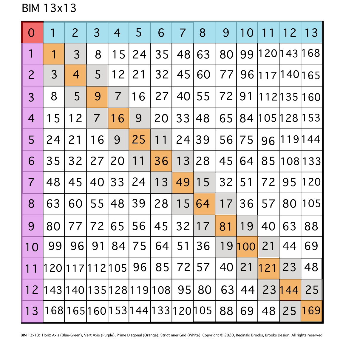Fig. 0.

TIP: The BIM is bilaterally (mirror) symmetric about the central diagonal in ORANGE.

TIP: The Inner Grid (IG) cell values — in WHITE or GRAY — are made up of the difference between the two diagonals (ORANGE) that intercept, e.i. 12 = 16-4.

TIP: The IG cell values alternate EVEN-ODD, all EVENS are ÷4, the Strict IG — exclude the GRAY — contains ALL the NO-PRIME ODD #s.

\1. Draw a DIAGONAL between the 10's found on each Axis.

Fig. 1

TIP: Diagonal lines between the SAME EVEN #s between the two Axis will intersect key cells whose coordinates will inform said EVENS.

\2. Note that there are 10 STEPS from one Axis to the other.

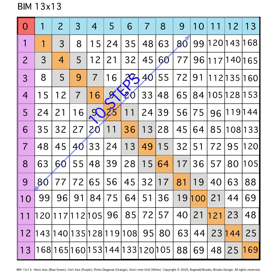Fig. 2

TIP: STEPS between similar Axis #s equal said Axis #.

\3. Halfway, at STEP 5, the DIAGONAL intersects the PD at 25.

Fig. 3

TIP: Dividing said EVEN Axis/2 = 1/2 the STEPS & intersects the Prime Diagonal (PD). The PD mirror divides the BIM.

\4. This PD 25 is the Square of 5 as 5•5, and 5,5 = PPset, as 5+5=10.

Fig. 4

TIP: The coordinates of the intersected PD — e.i., 5,5 — sum to equal the said EVEN, i.e., 10 in this example. The 5,5 is a PRIMES Pair set (PPset).

\5. At STEP 3 along the DIAGONAL, the intersect = 3,7 PPset, i.e., that BIM cell is located at the intersect of Column 7, Row 3, and 3+7=10.

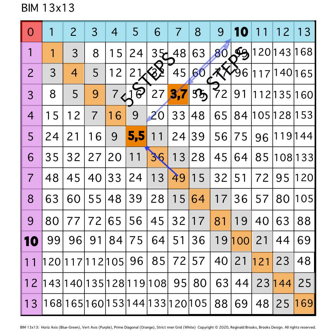Fig. 5

TIP: At 3 STEPS, the EVEN’s diagonal intersects another cell — 40 — whose coordinates 3,7 sum to equal said EVEN — 10.

\6. At STEP 7 along the DIAGONAL, the intersect = 3,7 PPset, i.e., that BIM cell is located at the intersect of Column 3, Row 7, and 7+3=10. 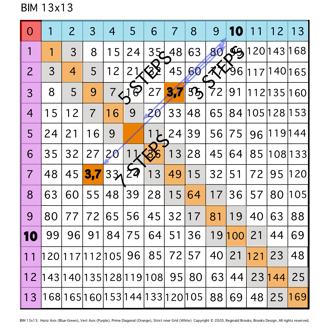Fig. 6

TIP: Being bilaterally symmetric, the EVEN’s Diagonal continues on to intersect another cell — 40 — on the lower symmetry, and, this is 7 STEPS in along the EVEN’s diagonal.

\7. Note the symmetry in no.5 and 6 above. On either side of the PD, there will always be a mirror-symmetrical PPset. By convention, the PPsets are listed with the smaller # first.

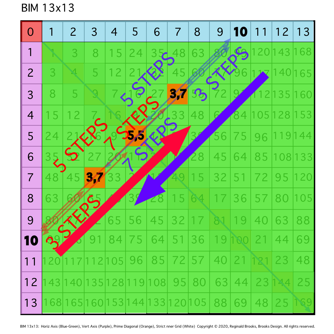Fig. 7

TIP: Sequentially counting the STEPS one way along the entire diagonal is mirrored in going the reverse direction, both revealing the intersected coordinates as PRIME Pair sets (PPsets) that sum up to equal said EVEN, i.e., 3+7 = 5+5 = 10.

\8. At the halfway PD 25, draw a vertical line up to the top Axis at 5 = 10/2.

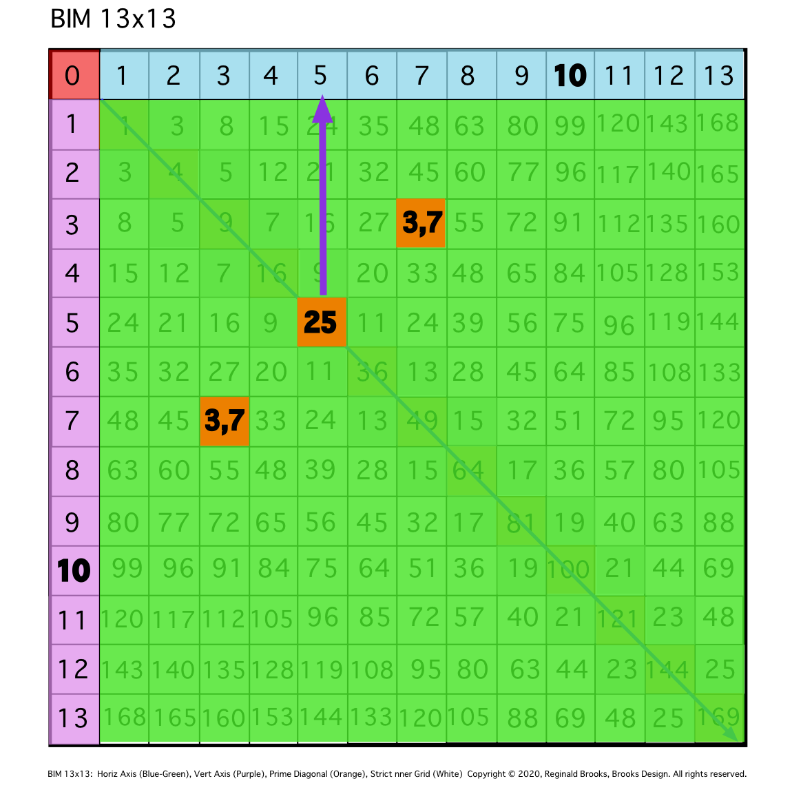Fig. 8

TIP: An ARROW up the intersecting PD (25 and 5,5 PPset) column points to the Axis that = said EVEN/2 as 10/2=5. It also points to one of the coordinates of the 5,5 PPset.

\9. Locate the Axis 3 and Axis 7 numbers, noting that they are 3 STEPS and 7 STEPS from the origin 0, and, that they are symmetrically located to either side of the Axis 5, that, in this case, happens to also be a PPset of 5,5.

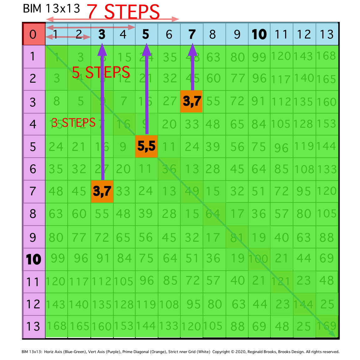Fig. 9a

TIP: ARROWS up from the other intersecting PPsets (symmetrical 3,7 PPsets) also point to their respective coordinates on the Axis, with the # of STEPS in from “0” noted.

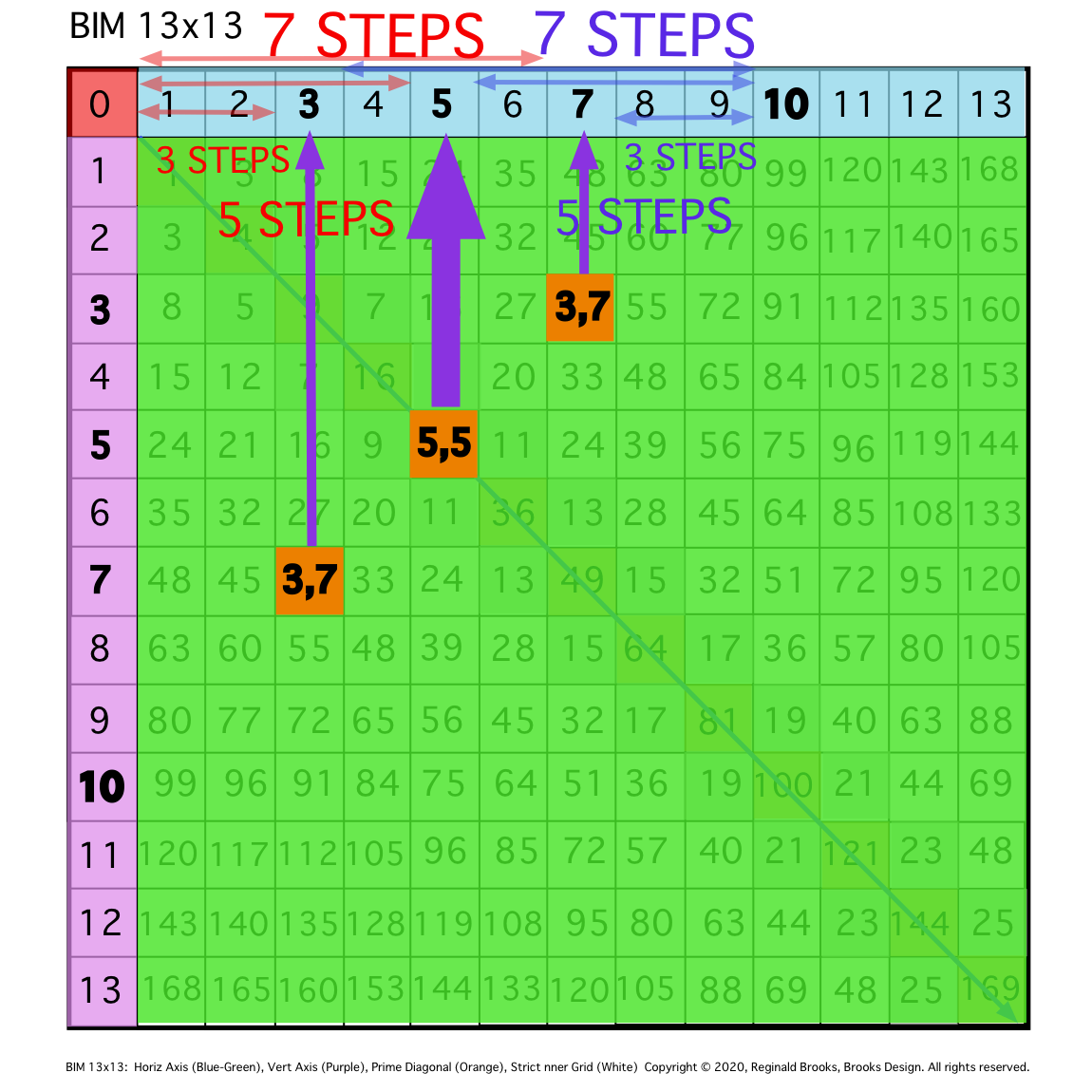Fig. 9b

TIP: The # of STEPS of the coordinates from the full EVEN value=10 back towards the central EVEN/2 = those coming forward — 3 STEPS & 5 STEPS.

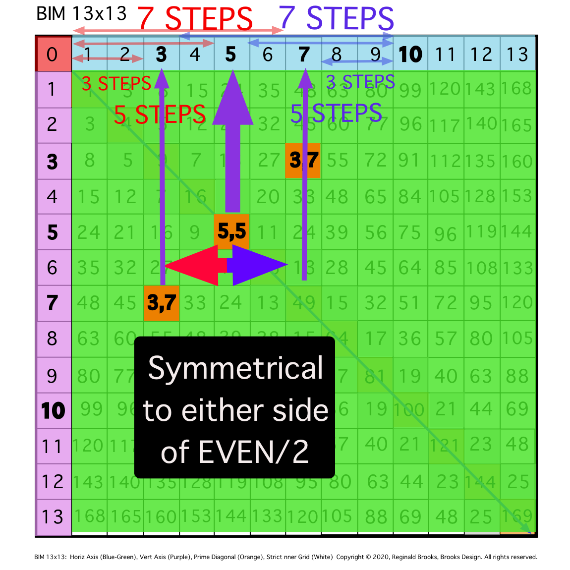Fig. 9c

TIP: The SYMMETRY of the PPset axial coordinates about the central EVEN/2 is one of the essential, defining relationship of ALL PPsets to the EVENS that they inform. The other is that they are formed and strictly follow the PRIMES Sequence Pattern as Fractals as shown on the Periodic Table Of PRIMES (PTOP). See references at the end.

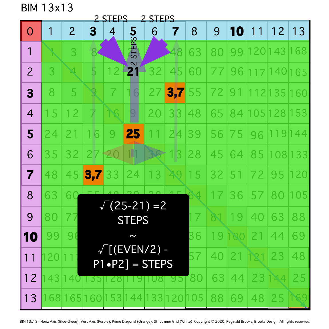Fig. 9d

TIP: An early finding that led to the PTOP and this whole simplification is that smaller diagonals from the Axial PPset coordinates form equilateral triangles whose apex intersects the original EVEN/2 central Column line at STEPS = the distance from the Axial coordinates to the said EVEN/2.

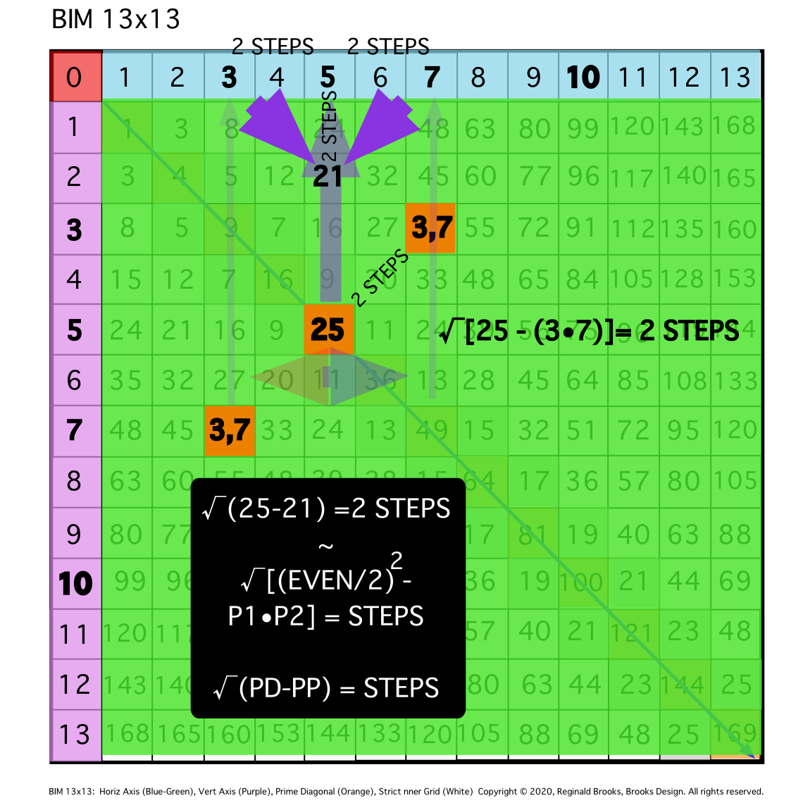Fig. 9e

TIP: The above can be described algebraically as: STEPS =√(PD - PPset product), e.i. STEPS = √(PD25 - product of PPset 3,7) = √4 = 2.

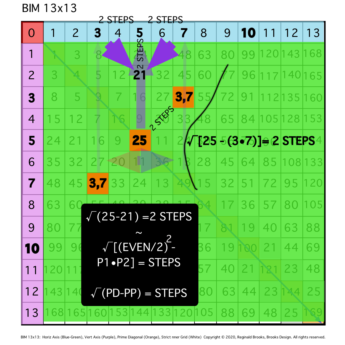Fig.9f

TIP: The addition of one free line ...

\10. ALL EVENS will follow this same PRIMES On the BIM (POB) pattern.

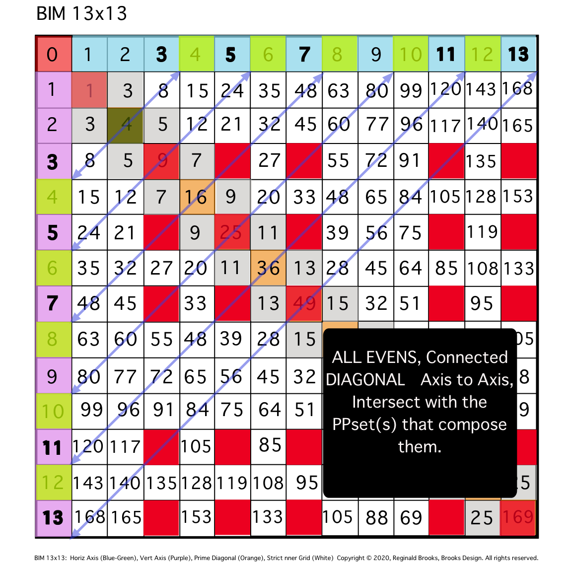Fig. 10a

TIP: SIMPLIFICATION: Diagonal lines from same Axial EVEN to Axial EVEN will intersect grid boxes whose Axial coordinate values sum to the said EVEN value.

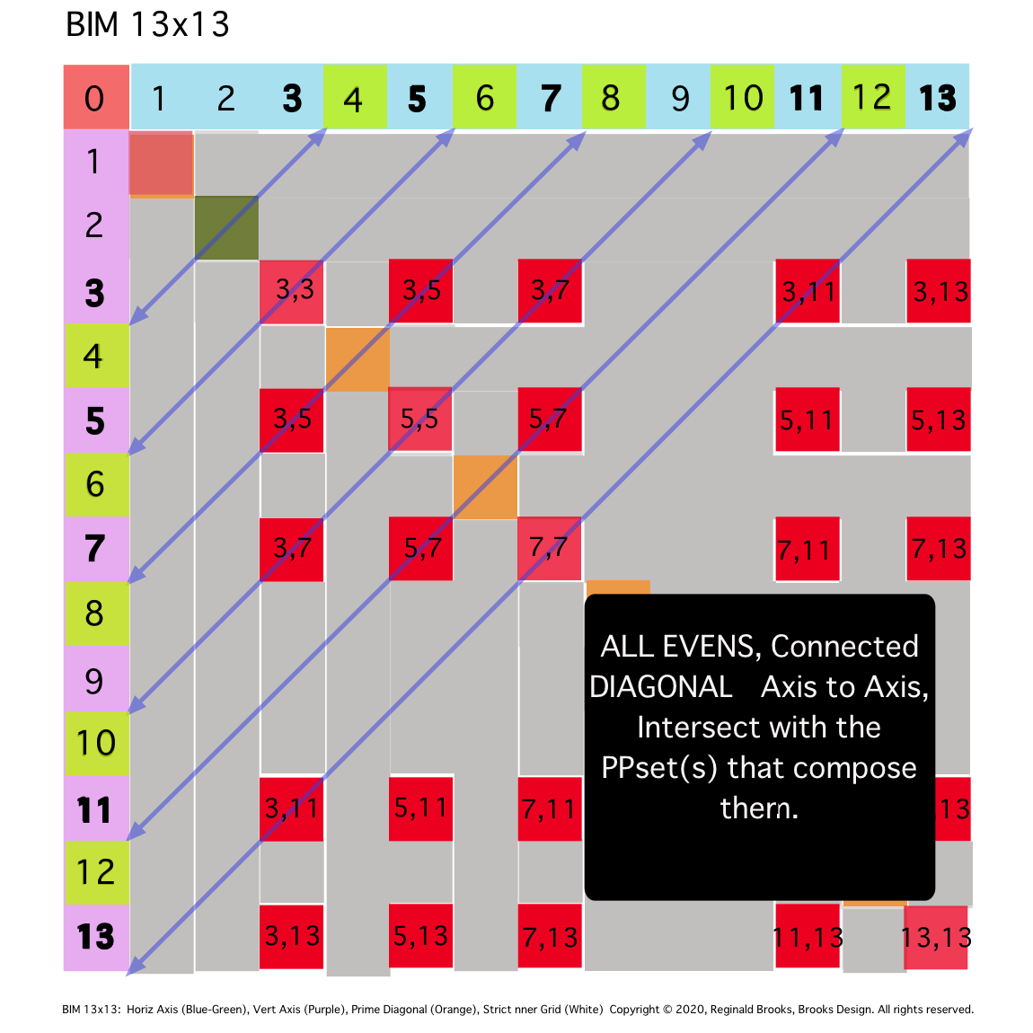Fig. 10b

TIP: SIMPLIFICATION: But first overlay the actual PPset values and gray-out the remaining grid. Diagonal lines from same Axial EVEN to Axial EVEN will intersect grid boxes whose Axial coordinate values sum to the said EVEN value.

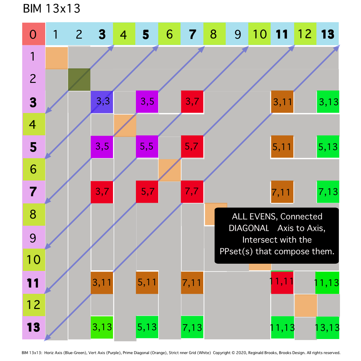Fig. 10c

TIP: SIMPLIFICATION: Diagonal lines from same Axial EVEN to Axial EVEN will intersect grid boxes whose Axial coordinate values sum to the said EVEN value. The expanding "Areas" are color coded.

Fig. 10d

TIP: SIMPLIFICATION: Diagonal lines from same Axial EVEN to Axial EVEN will intersect grid boxes whose Axial coordinate values sum to the said EVEN value. Fill-in grid lines and we have a simple working copy.

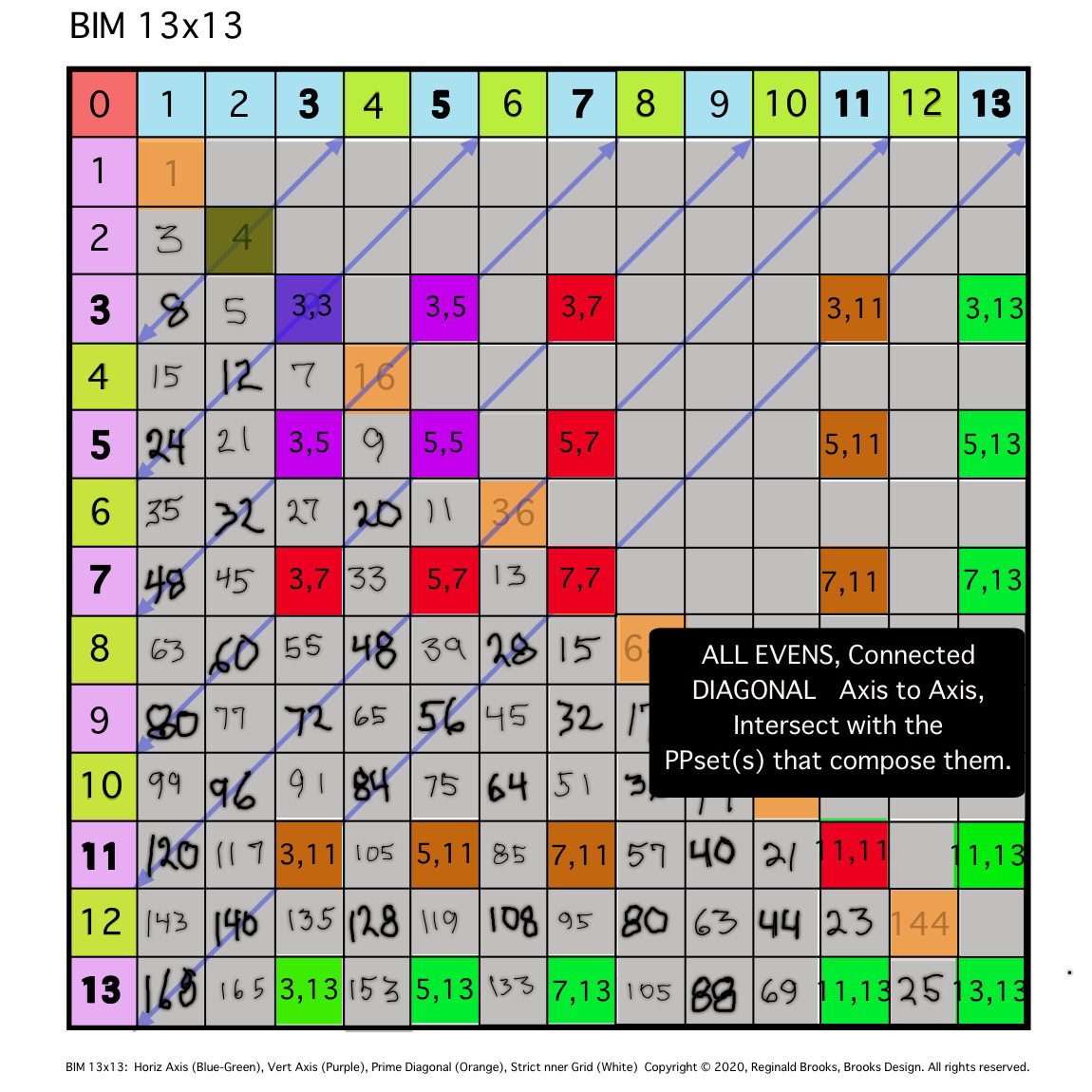Fig. 10e

TIP: SIMPLIFICATION: Diagonal lines from same Axial EVEN to Axial EVEN will intersect grid boxes whose Axial coordinate values sum to the said EVEN value. To this one can use markup to fill in the grid cell values as needed.

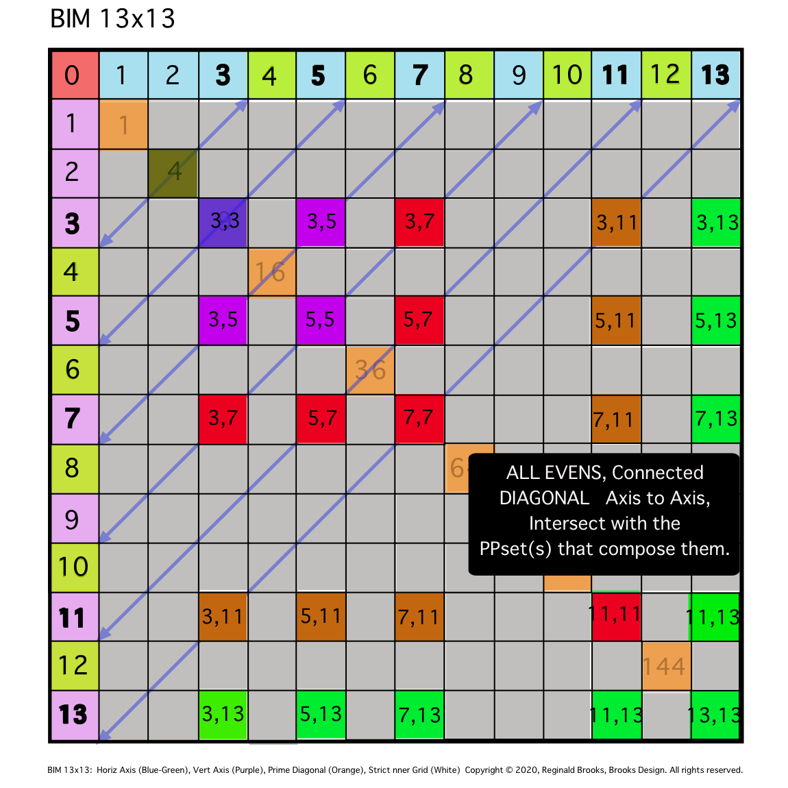Fig. 10d reference

TIP: Try using markup to fill in the BIM! It will be useful!

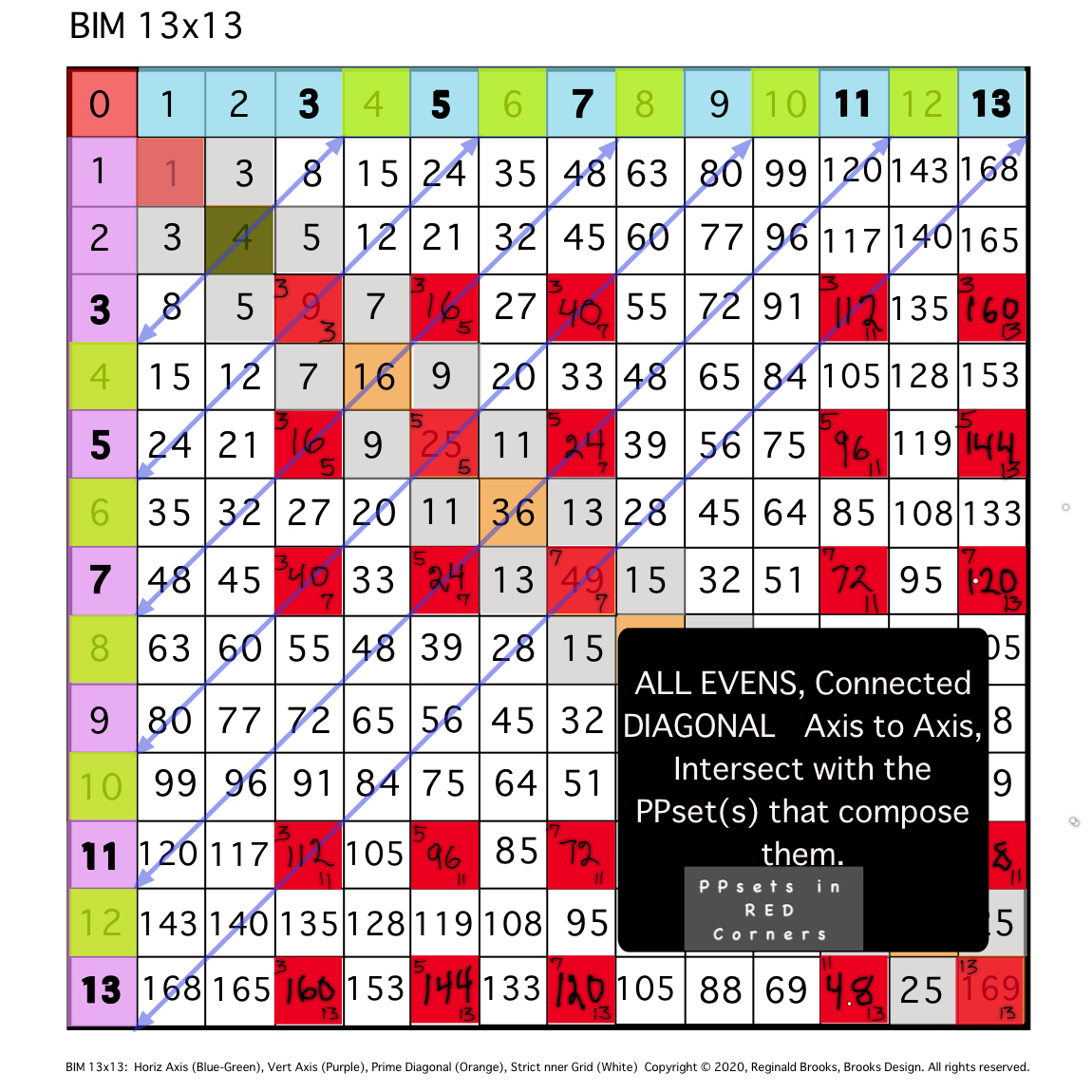Fig. 10f Reference

TIP: Try using markup to fill in the BIM! Here is reference example.

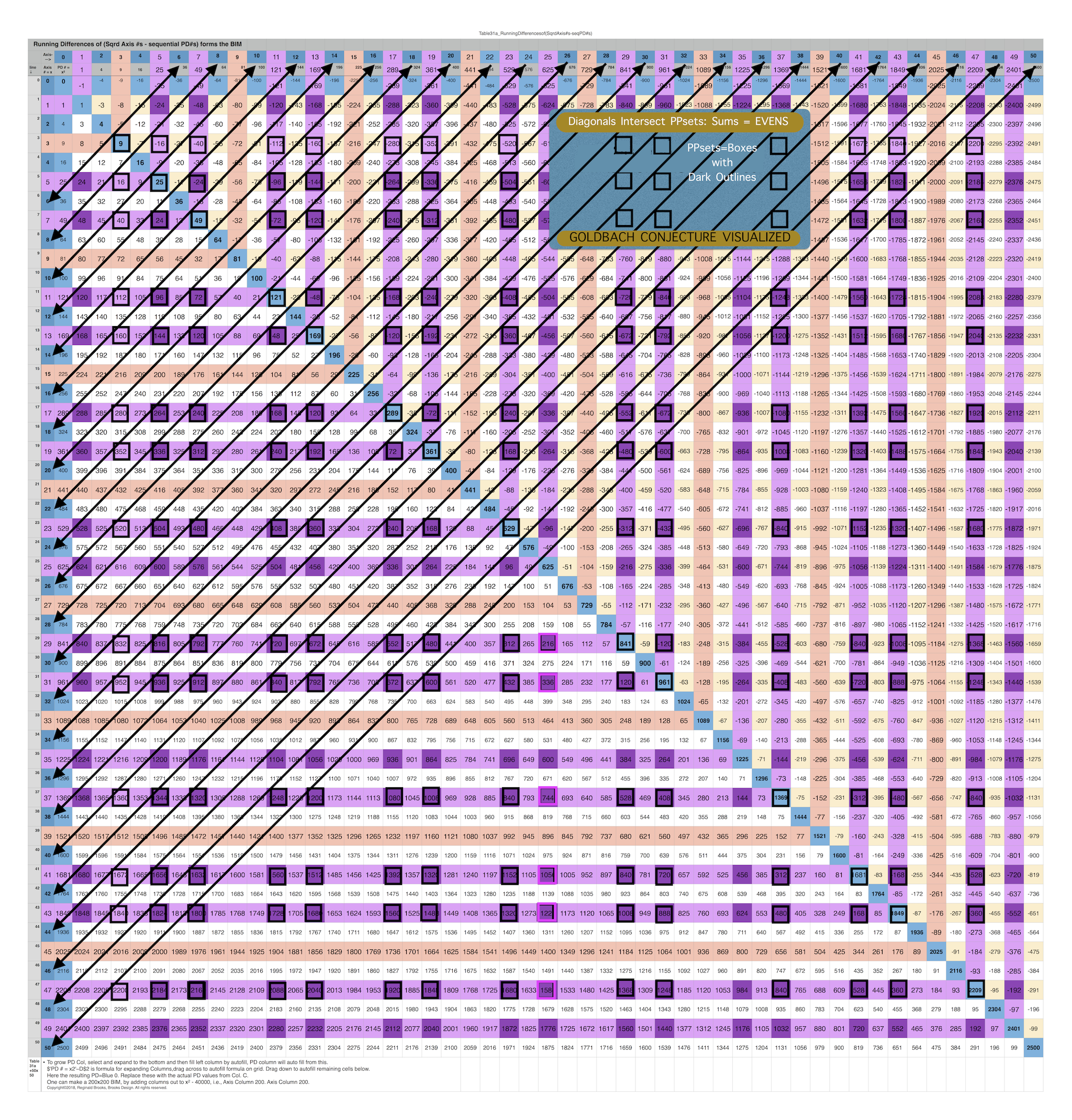Fig. 10g Reference Large (50x50)

TIP: Try using markup to fill in the BIM! Here is reference example.

Fig. 10g Reference Large (50x50)

TIP: Try using markup to fill in the BIM! Here is PDF reference example.

Fig. 10h Reference PPsets Large (50x50)

TIP: Try using markup to fill in the BIM! Here is reference example.

Fig. 10h Reference PPsets Large (50x50)

TIP: Try using markup to fill in the BIM! Here is PDF reference example.

Here are all the TIPS:

• TIP: The BIM is bilaterally (mirror) symmetric about the central diagonal in ORANGE.
• TIP: The Inner Grid (IG) cell values — in WHITE or GRAY — are made up of the difference between the two diagonals (ORANGE) that intercept, e.i. 12 = 16-4.
• TIP: The IG cell values alternate EVEN-ODD, all EVENS are ÷4, the Strict IG — exclude the GRAY — contains ALL the NO-PRIME ODD #s.
• TIP: Diagonal lines between the SAME EVEN #s between the two Axis will intersect key cells whose coordinates will inform said EVENS.
• TIP: STEPS between similar Axis #s equal said Axis #.
• TIP: Dividing said EVEN Axis/2 = 1/2 the STEPS & intersects the Prime Diagonal (PD). The PD mirror divides the BIM.
• TIP: The coordinates of the intersected PD — e.i., 5,5 — sum to equal the said EVEN, i.e., 10 in this example. The 5,5 is a PRIMES Pair set (PPset).
• TIP: At 3 STEPS, the EVEN’s diagonal intersects another cell — 40 — whose coordinates 3,7 sum to equal said EVEN — 10.
• TIP: Being bilaterally symmetric, the EVEN’s Diagonal continues on to intersect another cell — 40 — on the lower symmetry, and, this is 7 STEPS in along the EVEN’s diagonal.
• TIP: Sequentially counting the STEPS one way along the entire diagonal is mirrored in going the reverse direction, both revealing the intersected coordinates as PRIME Pair sets (PPsets) that sum up to equal said EVEN, i.e., 3+7 = 5+5 = 10.
• TIP: An ARROW up the intersecting PD (25 and 5,5 PPset) column points to the Axis that = said EVEN/2 as 10/2=5. It also points to one of the coordinates of the 5,5 PPset.
• TIP: ARROWS up from the other intersecting PPsets (symmetrical 3,7 PPsets) also point to their respective coordinates on the Axis, with the # of STEPS in from “0” noted.
• TIP: The # of STEPS of the coordinates from the full EVEN value=10 back towards the central EVEN/2 = those coming forward — 3 STEPS & 5 STEPS.
• TIP: The SYMMETRY of the PPset axial coordinates about the central EVEN/2 is one of the essential, defining relationship of ALL PPsets to the EVENS that they inform. The other is that they are formed and strictly follow the PRIMES Sequence Pattern as Fractals as shown on the Periodic Table Of PRIMES (PTOP). See references at the end.
• TIP: An early finding that led to the PTOP and this whole simplification is that smaller diagonals from the Axial PPset coordinates form equilateral triangles whose apex intersects the original EVEN/2 central Column line at STEPS = the distance from the Axial coordinates to the said EVEN/2.
• TIP: The above can be described algebraically as: STEPS =√(PD - PPset product), e.i. STEPS = √(PD25 - product of PPset 3,7) = √4 = 2.
• TIP: The addition of one free line ...
• TIP: SIMPLIFICATION: Diagonal lines from same Axial EVEN to Axial EVEN will intersect grid boxes whose Axial coordinate values sum to the said EVEN value.
• TIP: SIMPLIFICATION: But first overlay the actual PPset values and gray-out the remaining grid. Diagonal lines from same Axial EVEN to Axial EVEN will intersect grid boxes whose Axial coordinate values sum to the said EVEN value.
• TIP: SIMPLIFICATION: Diagonal lines from same Axial EVEN to Axial EVEN will intersect grid boxes whose Axial coordinate values sum to the said EVEN value. The expanding "Areas" are color coded.
• TIP: SIMPLIFICATION: Diagonal lines from same Axial EVEN to Axial EVEN will intersect grid boxes whose Axial coordinate values sum to the said EVEN value. Fill-in grid lines and we have a simple working copy.
• TIP: SIMPLIFICATION: Diagonal lines from same Axial EVEN to Axial EVEN will intersect grid boxes whose Axial coordinate values sum to the said EVEN value. To this one can use markup to fill in the grid cell values as needed.
• TIP: Try using markup to fill in the BIM! It will be useful!

​

What we are seeing here is a distillation and reconfiguration of:

• • Periodic Table of PRIMES (PTOP)
  • PTOP on the BIM
  • PRIMES on the BIM

into a new simplified whole proof of Euler's Strong Form of the Goldbach Conjecture.

On the BIM the original PTOP, PTOP on the BIM and PRIMES on the BIM PPsets are juxtaposed with the visual proof of a given EVEN #.

Overlaid upon this, and the really new simplification, are the perpendicular DIAGONALS between the Axis EVENS. These DIAGONALS streamline the connections between the EVENS and their symmetrically distributed PPsets that inform them. It is no small wonder that the number of STEPS down (or up) the diagonal to each PPset matches their location on the AXIS!

Summary

As the PTOP has shown that the number of PPsets growth rate exceeds the PRIMES span rate, combined with the infinite distribution of the PPset within the infinite expansion of the BIM itself, we can say with confidence that:

Every EVEN # (≥2, or include 2 if you consider 1 to be prime, as the ancients did) is composed of one or more pair sets of PRIMES.

And in its most simplified restatement:

On the BIM, DIAGONALS between Axial EVENS intersect their composing PPsets.

~~~~~~~~~~~~~~~~~~~~~

(NOTE: The following section contains NEW material and as such, it introduces some new content and complexity to the mix!)

Something NEW!

AREAS & VOLUMES (the latter as Cubed Areas) on the BIM predict the NEXT PRIMES

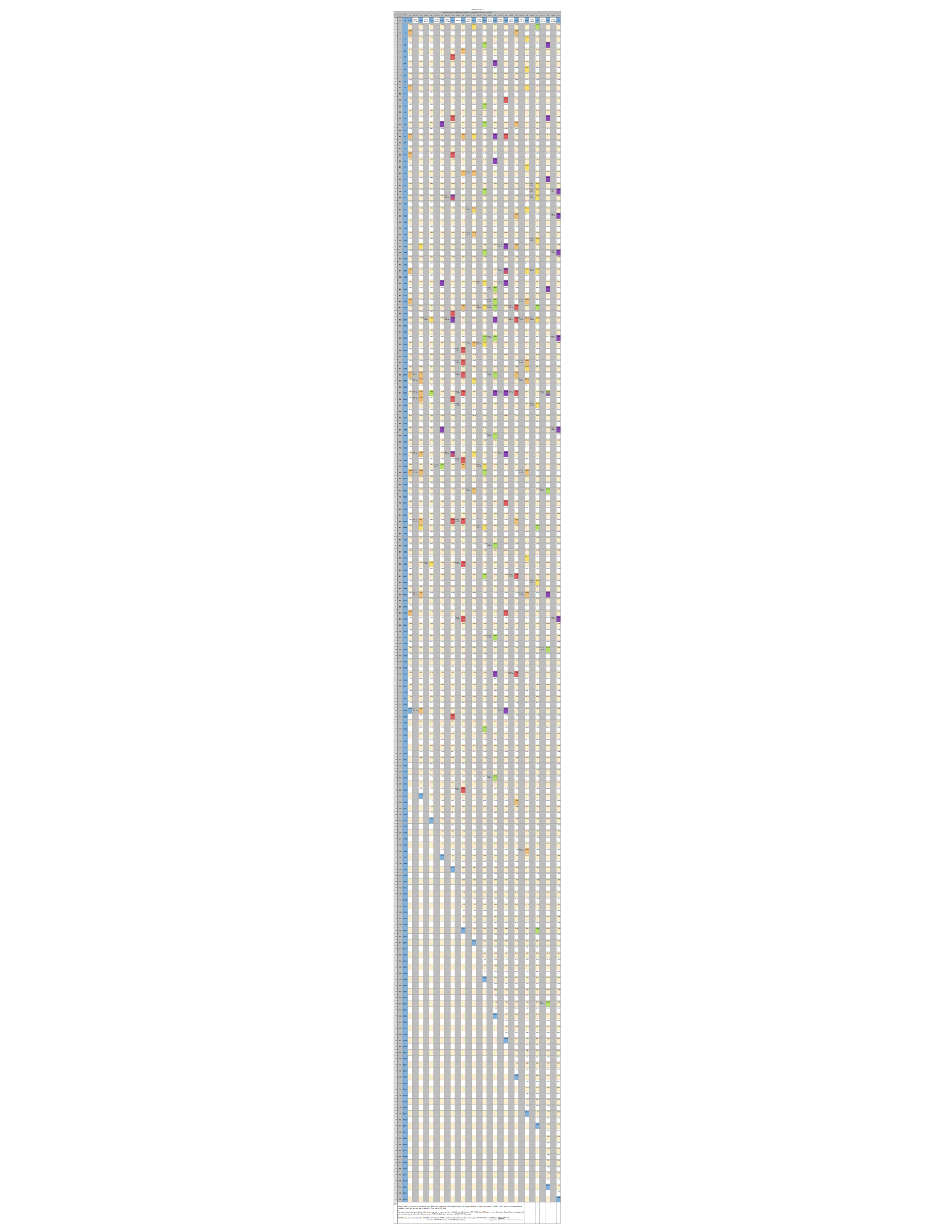
Table 31a

Table31a_+RunningDifferencesof+50x50+.png

An interesting visual emerges when we do a slight alteration to Table 31a . This graphic table shows the Active Rows. Eliminating the Col/Rows 1, 25, 35 (45 is done already), and, adding RED grid cells for Col/Row 3, reveals the PPsets and the remarkable pattern they form on the BIM. We have already seen a slightly refined version of this above the Summary.

On the BIM, the ∆ in cell values between Rows 1 STEP apart is 1 STEP in from the PD; Rows 2 STEPS apart are 2 STEPS in from the PD, 3 STEPS apart, 3 STEPS in,... The ∆ remains true for all cells across any given Row. This is built in to the BIM.

For example, going from 16 on Row 5 to 40 on Row 7 has a ∆ = 24 and that 24 is found 2 STEPS in from the PD. The ∆ is always just the ∆ between the vertical Column and horizontal Row PD intersects. Here in this example between PD 49 on Row 7 and PD 25 on Column 5. This holds true for every cell on the BIM.

Remarkably, the PPsets not only follow the pattern, they also reproduce their own PRIME Sequence Pattern in do so! How so?

The PPsets, being symmetrical to the BIM, reproduce their own PRIME Sequence Pattern both across and down the BIM.

Table 31a Altered

Table 31a Altered twice BIM50x50-PPsets-Table31a_Anno_Right and Left with Diag PDF overview

BIM50x50-PPsets-Table31a_Anno_LEFT with Diag

BIM50x50-PPsets-Table31a_Anno_LEFT.pdf

The BIM is bilaterally-mirror symmetric. If you have a pattern that runs both down a Column and across a Row on one symmetry side, it mirror reflects into an equal but opposite Row and Column on the other side -- like a Square (Rectangle) -- giving the remarkable PPsets PRIME Sequence Pattern.

When you look at the ∆ in STEPS between the PPsets you really see this dual symmetry in action, e.i. if you go from the 3,5 PPset (16) down to the 3,11 PPset (112) in 6 STEPS, you find that at 6 STEPS in from the PD 121 is found the 96 cell housing the cell ∆ (112–16=96) of the 3,5 and 3,11 PPsets.

Because the vertical Column pattern in the lower symmetry side (3,3--3,5--3,7--3,11) mirrors the same, only as a horizontal Row on the upper symmetry side, when we count the STEPS on the lower, they equal the STEPS on the upper, and, they do so in the SAME PRIMES Sequence Pattern. Down from the PD, in from the PD.

BIM50x50-PPsets-Table31a_Anno_Right swith Diag

BIM50x50-PPsets-Table31a_Anno_RIGHTwithDiagAR.pdf

Notice (Large Black Arrows on BIM50x50-PPsets-Table31a_Anno_Rightwith Diag.jpeg and pdf) that the going down vertical pattern of PPsets in the lower symmetry (set-STEP-set-STEP-set-STEP-STEP-STEP-set-STEP-set-STEP-STEP-STEP-set-STEP...) is exactly repeated going across the Row(s). And, of course, that includes going across the Row(s) in the upper symmetry.

Yet, when we are calculating the ∆ in the cell values going down the Rows (Columns) by counting the STEPS from Row to Row, we obtain that ∆ by going back in from the PD in the same number of STEPS to get the cell ∆ value!

The PPset pattern (PRIMES Sequence Pattern) goes Down and Across toward the PD in the lower symmetry, while the STEPS go Down and Across back-in, away from the PD, to locate the cell ∆ value. And, in every case, it will always land on a PPset!

For example, take the 3,7 PPset (cell = 40) and drop down to the 3,11 PPset (112) in 4 STEPS. Now, from the PD on the 3,11 PPset Row at 121, come back-in across the Row -- away from the PD -- 4 STEPS, landing on the 7,11 PPset (72) that is the cell ∆ between 112 and 40. The PPset pattern as a whole PRIMES Sequence Pattern going Down the BIM is mirrored going Across the BIM, while the STEPS pattern going Down the BIM goes Across the BIM in the Reverse direction -- yet always lands on a PPset.

It is no coincidence that in coming away from the PD, reversing across the Row the same number of STEPS lands on a PPset with the exact cell ∆ value!

You can see how this is so by taking it to the extreme. Instead of starting with the 3,7 PPset, go all the way up to the 3,3 PPset that actually sits on the PD 9. Note the STEPS from 3,3 to 3,11 equals 8, and the STEPS back-in from the PD 121† to 3,11 equals 8, and here we find the defining cell ∆ between the Rows as ultimately the ∆ between PD 121 and PD 9, or 112. It is very helpful to "see" these patterns and pathways on the colored Areas of the PPsets PRIMES Sequence Pattern on the graphic table.

This works universally across the BIM.

Now for the significance.

Knowing the previous PRIMES Sequence Pattern allows one to predict the NEXT in the series! Knowing that ALL PRIMES within the PRIMES Pattern Sequence must land on -- and only on -- Active Rows (ODD Rows NOT ÷ 3) gives a pathway to revealing ALL PRIMES! But wait, there is more! Something very new that adds to the predictability.

TABLE 54

Table54_PPsetAreaPatterns+Goldbach.pdf

TABLE 55

Table55_BIM-GB_IG_sheets-1-3.pdf

Table55_BIM-GB_IG_sheets-1.pdf

Table55_BIM-GB_IG_sheets-2.pdf

~~~~~~~

PERIMETERS & AREAS on the BIM

Well, not really the Perimeter, P, but rather a length = Axis Row # = Ax

Square Areas are the Ax² = Axis Row #²

Area, A = 4Ax + nAx, where n=…–3,2,1,0,1,2,3,… n=0 @ Ax=4 and x=1,4,9,16,25,...

ALL SQUARE AREAS equal the SUM of 4Ax + nAx.

Fig. 11a

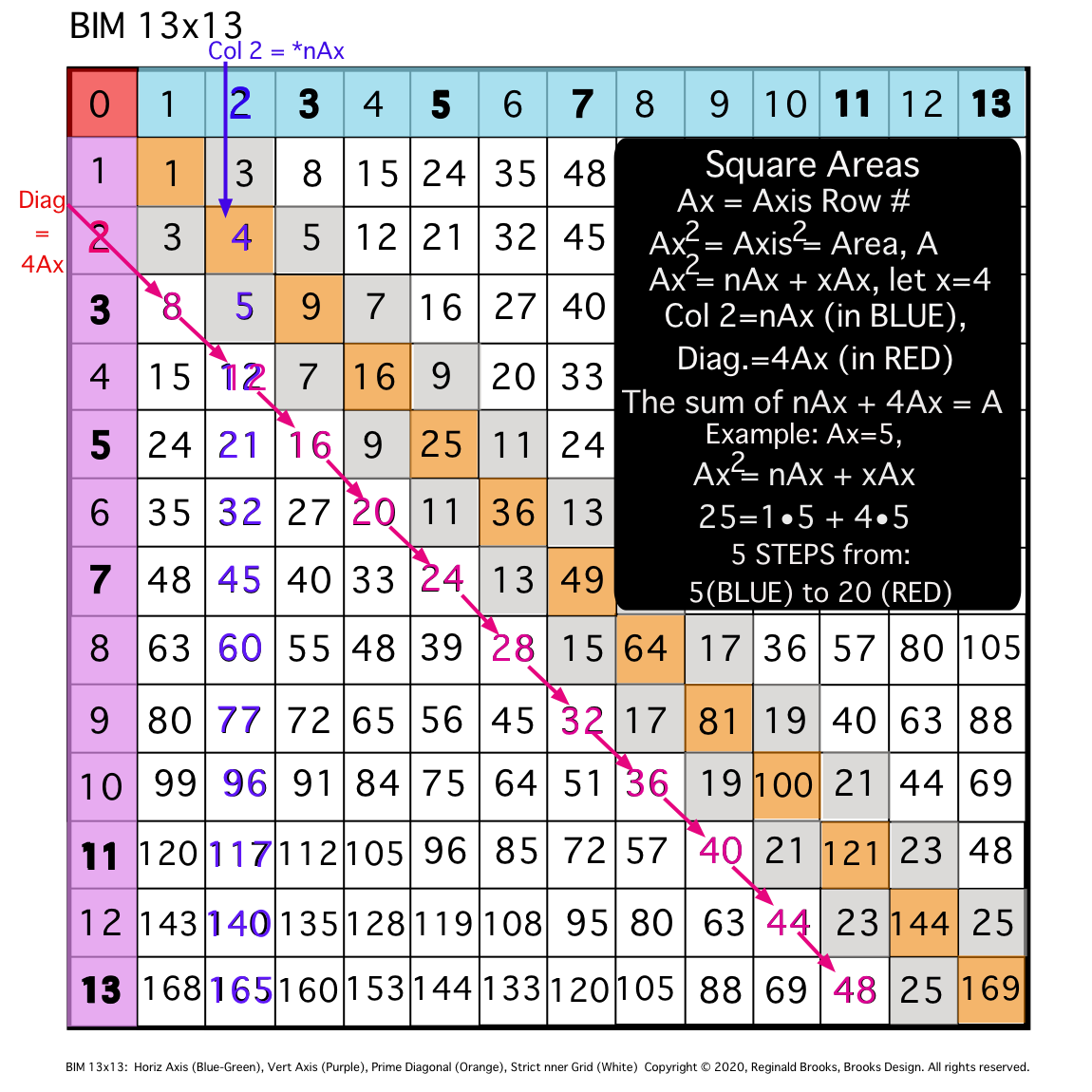
 Fig. 11b

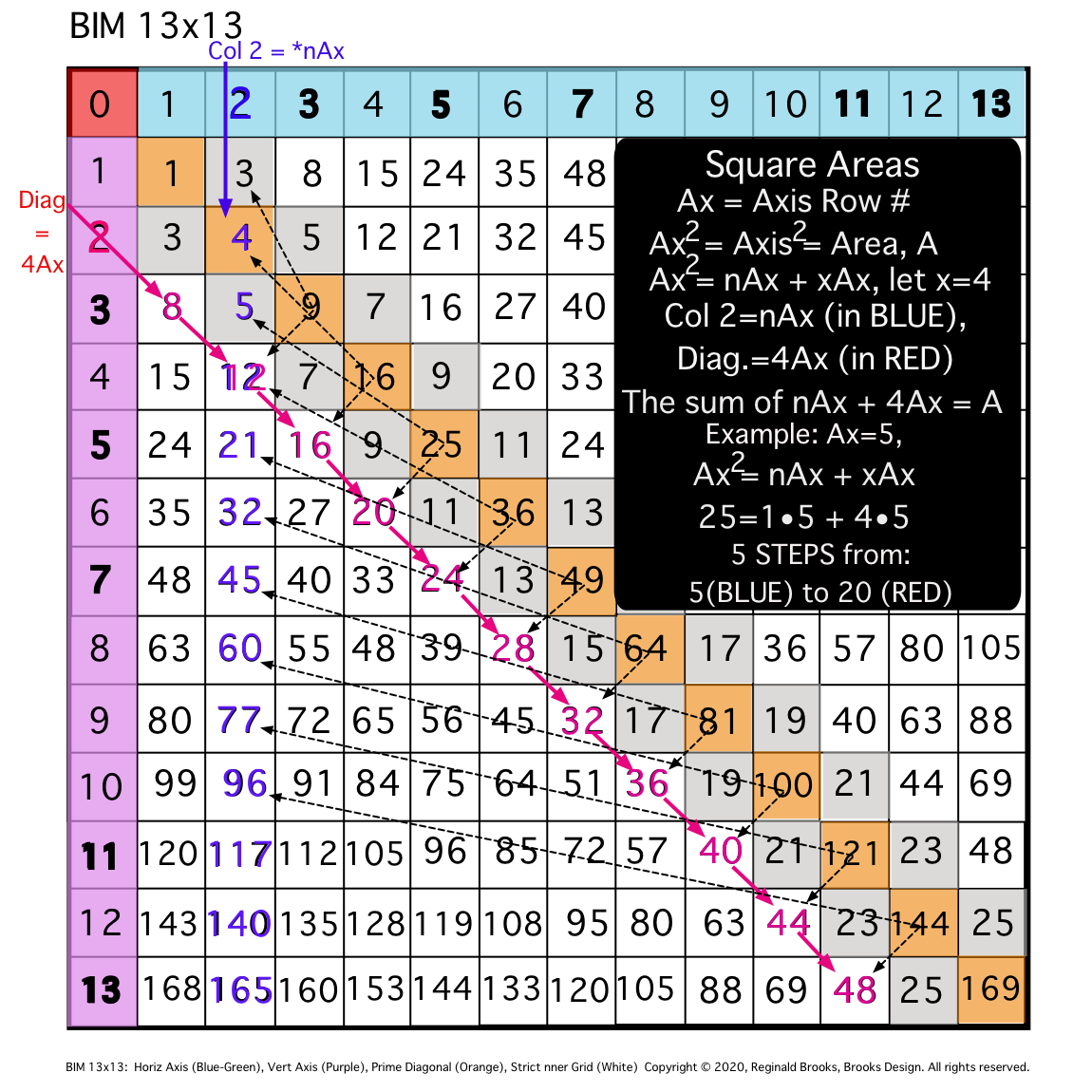Fig. 11c

Ax²= A = 4Ax + nAx**

• 1² = 1 = 4(1) - 3(1) = 4–3 = 1
• 2² = 4 = 4(2) - 2(2) = 8–4 = 4
• 3² = 9 = 4(3) –1(3) = 12–3 = 9
• 4² = 16 = 4(4) + 0(4) = 16+0 = 16
• 5² = 25 = 4(5) + 1(5) = 20+5 = 25
• 6² = 36 = 4(6) +2(6) = 24+12 = 36
• 7² = 49 = 4(7) + 3(7) = 28+21 = 49
• 8² = 64 = 4(8) + 4(8) = 32+32 = 64
• 9² = 81 = 4(9) + 5(9) = 36+45 = 81
• 10² = 100 = 4(10)+6(10) = 40+60 = 100

When plotted on the BIM:

1. All nAx are found on Col 2.
2. Starts with 4=nAx=0(4) = 0 and not on the Inner Grid, but PD4 is present.
3. nAx=4 occupies a pivotal spot on the BIM grid as n=0 for Ax=4, and n=–1 for Ax=3, n=–2 for Ax=2, n=–3 for Ax=1.
4. A Number Pattern Sequence (NPS) is seen in Column 2=nAx, as Ax=1,2,3,4,5,6,7..., n=–3,–2,–1,0,1,2,3,...respectively.
5. The Axis Row of nAx=Ax–2, e.i., for Ax=8, Axis Row is 8–2=6.
6. Add constant 3 STEPS down for the 4Ax Axis Row.
7. The 2^nd Parallel Diagonal -- starting with 8–12–16 -- sequentially holds all the 4Ax.
8. The Axis Row for the 4Ax=Ax+1, e.i., Ax=8, Axis Row for 4Ax Diagonal is 8+1=9, Row 9.
9. The # of STEPS across the Row = Ax–1, e.i., for Ax=8, 8–1=7 STEPS from Row Axis 9 over to cell=32=4(8)=4Ax.
10. The NPS for the STEPS across the Axis Row to the DIAGONAL cell increments by 1 as the DIAGONAL cell values increment by a constant 4, e.i. 8–12–16–20–24..., starting with 4Ax=8 and 1 STEP over from Row Axis 3, then 4Ax=12 and that is 2 STEPS across Row Axis 4 to cell =12, then 4Ax=16 and that's 3 STEPS across Row Axis 5 to cell = 16....
11. The Area of 4Ax -- beyond the pivotal Ax=4 -- is naturally a non-Square Rectangle with a constant 4 Rows x 5+ Columns.
12. The addition of the nAx Area fills out the 4Ax Rectangle to a full Square, as A=4Ax+nAx, e.i. for Ax=8 and 4Ax=32=4 Rows of 8 Columns giving a 32 cell Rectangle, and now adding the nAx=4(8)=32 Area, the total Area = 32 + 32 = 64 = 4Ax+nAx= full Square Area of 8²=64.

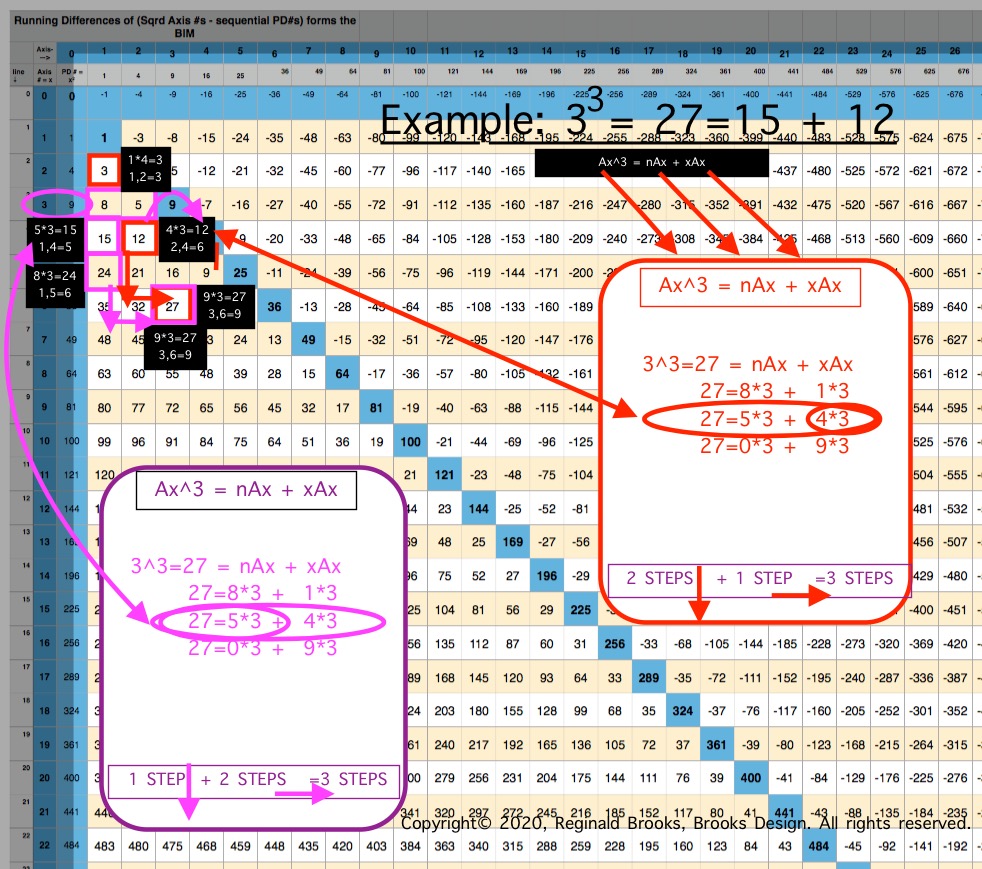
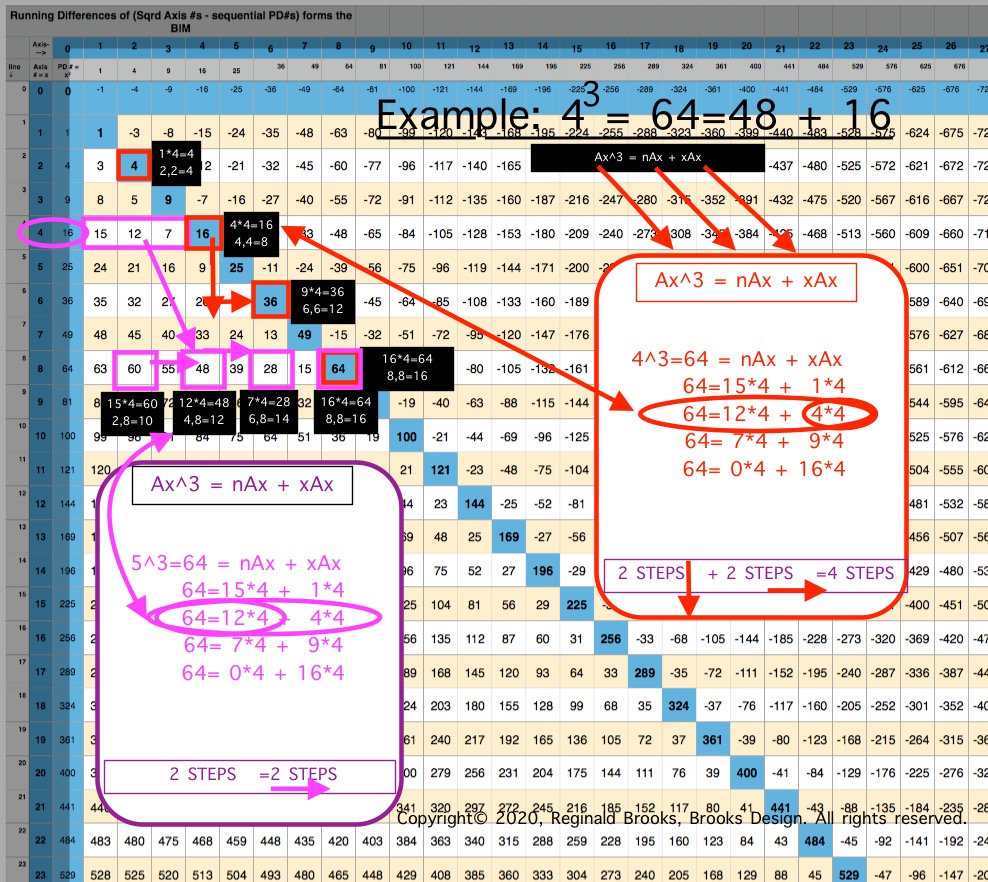
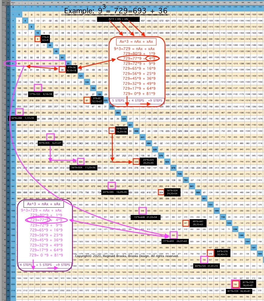
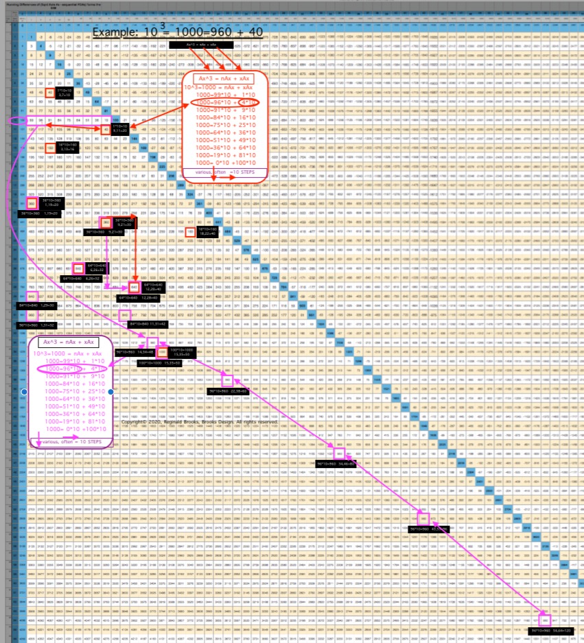
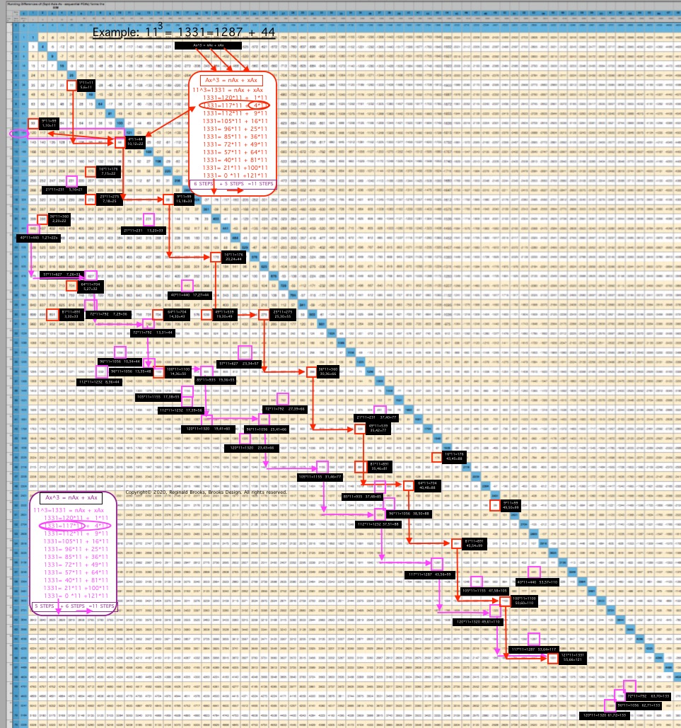
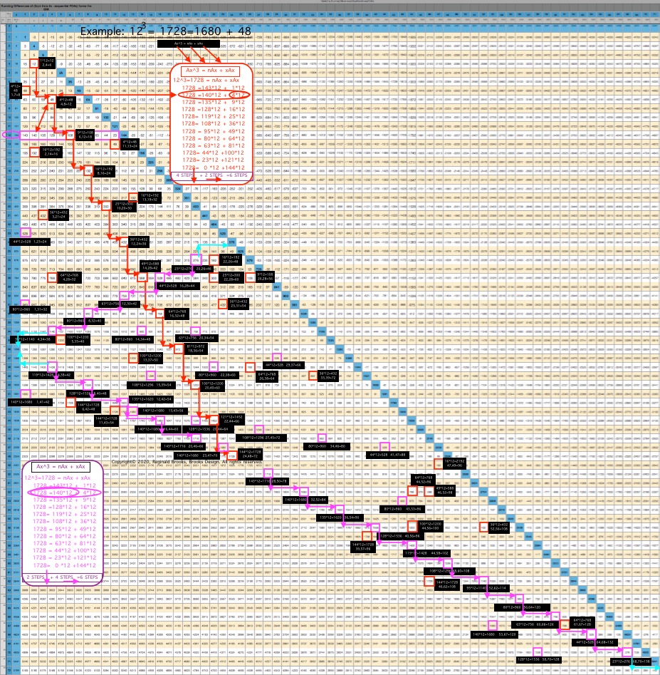
Table 56.

 Table56_SquareAreasOnBIM.pdf

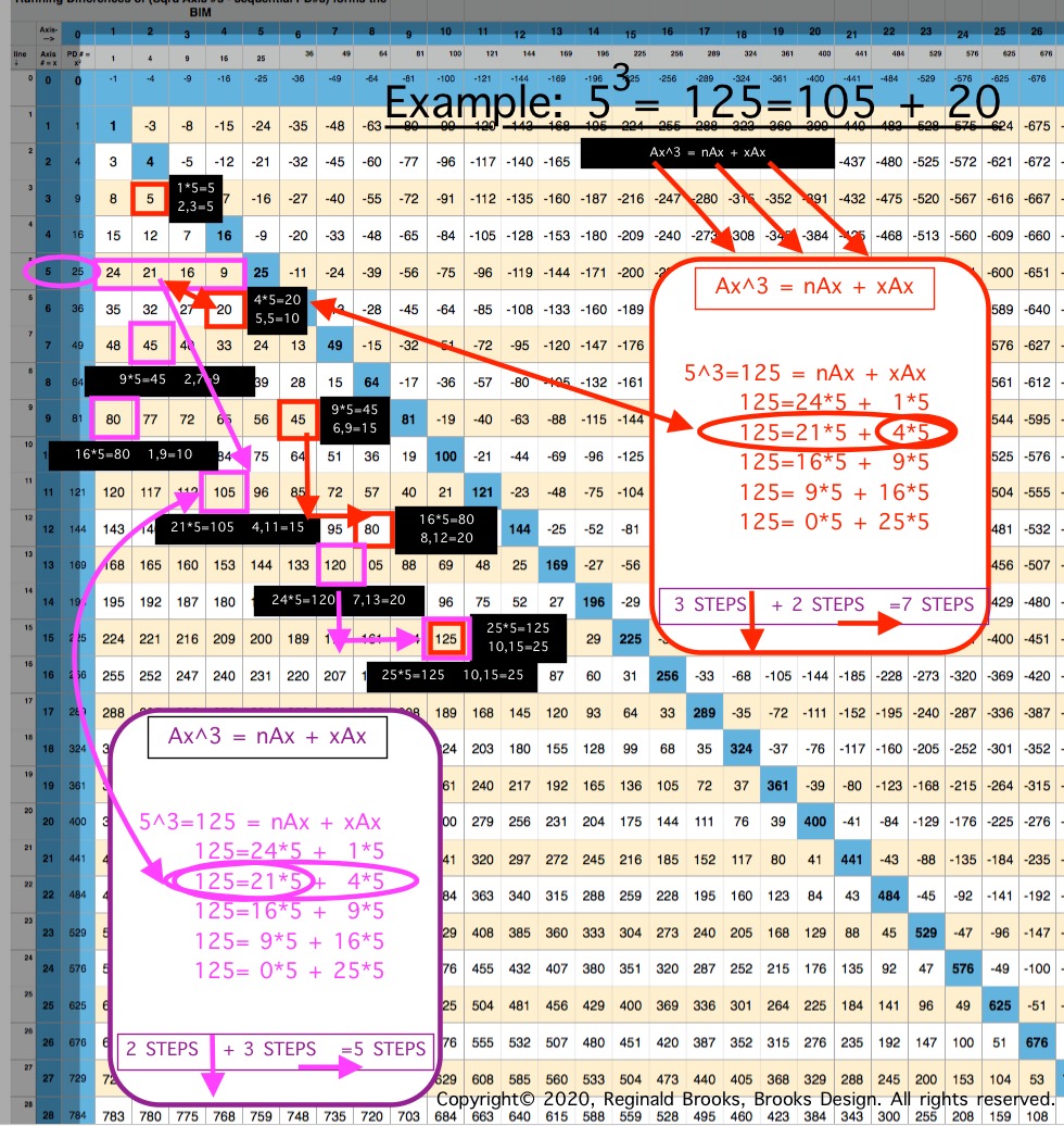
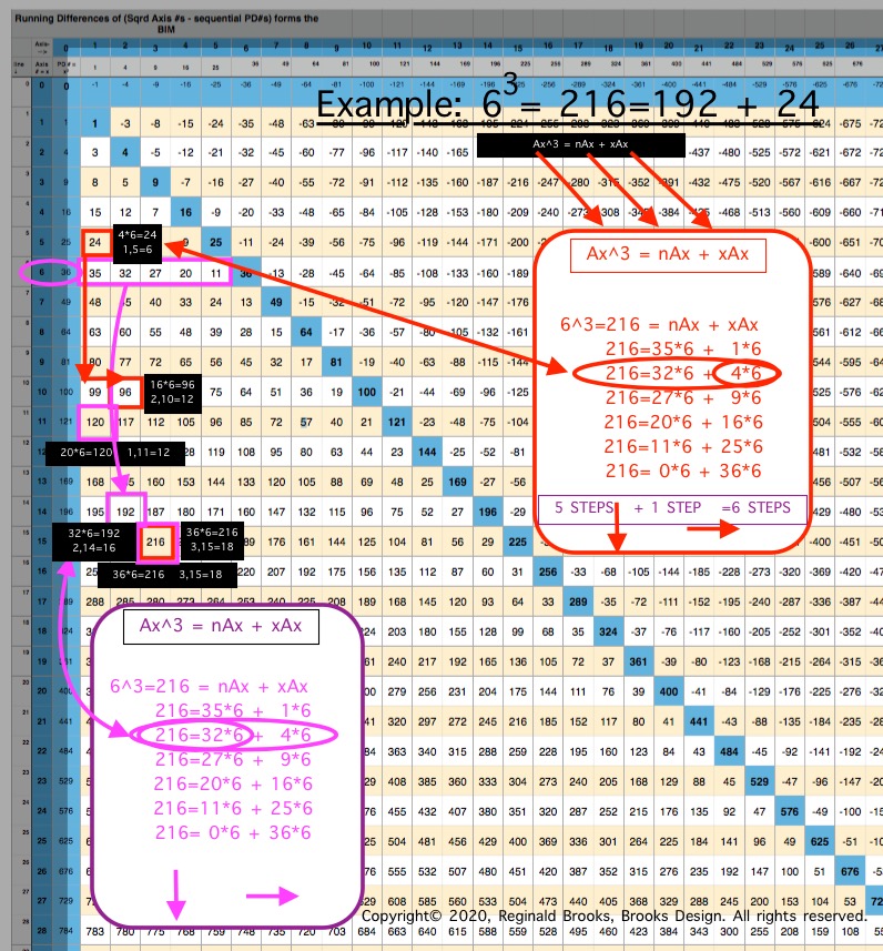
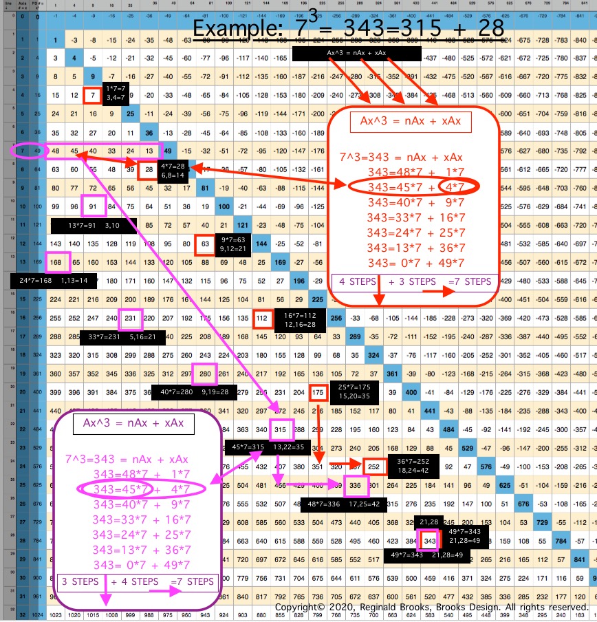
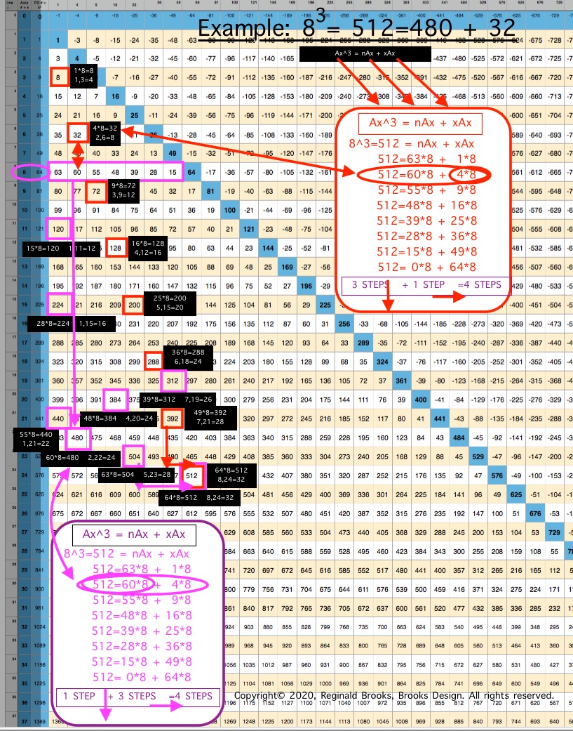
ALL CUBED AREAS equal the SUM of xAx + nAx (similar to SQUARES 4Ax + nAx, but with variable "x." Cubed Areas are the Ax³ = Axis Row #³. Commonly referred to as Volume (V), it is just the Area x (Ax) as (Ax²• Ax¹=Ax³).

Cubed Areas

Fig. 12a

Fig. 12b

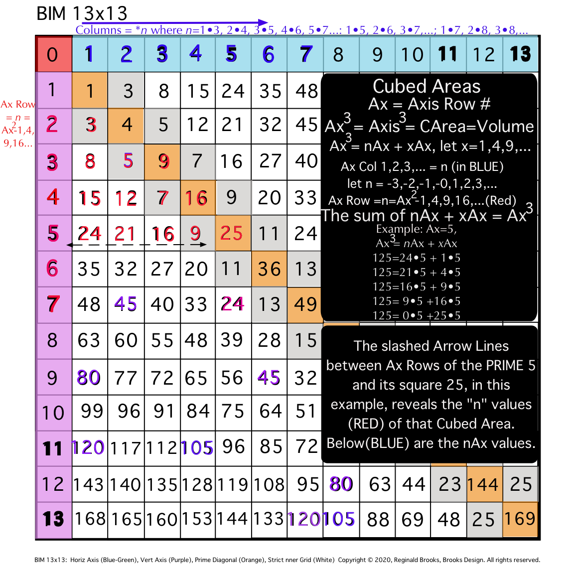Fig. 12c

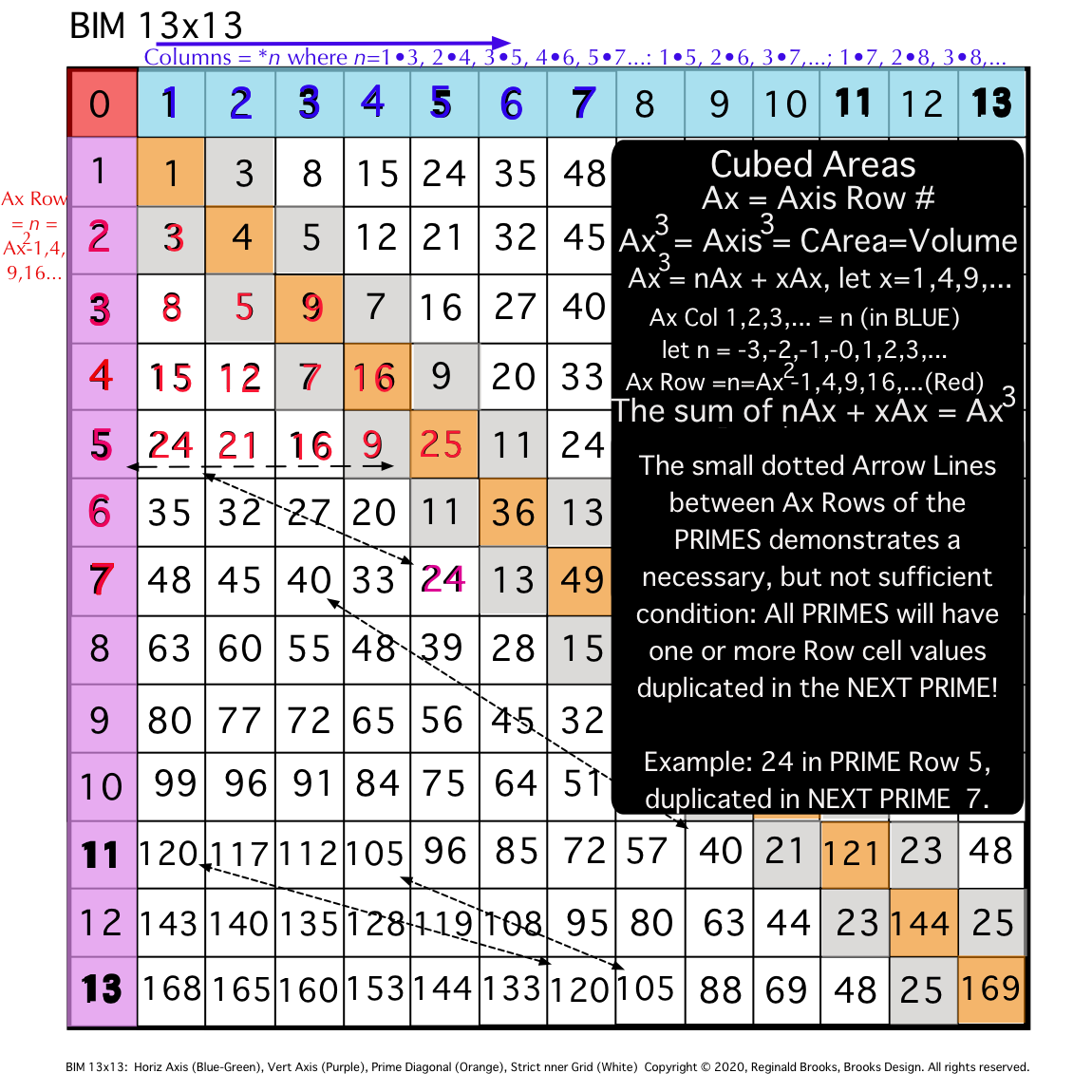Fig. 12d

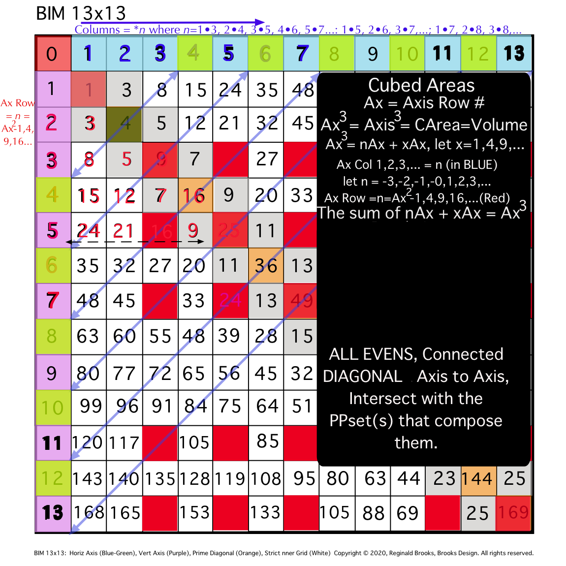Fig. 12e

Table 57.

Table57_CubedAreasOnBIM.pdf

The "x" variable in the Cubed Areas formula is crucial as now the BIM is reflecting the 1,4,9,16,25,... ISL sequence as "x."

Whereas in the Square Areas with the "x" = 4 -- giving the constant 4Ax value with 4 being the constant -- gives a single Column 2 value list for all Square Areas as the PRODUCT of nAx + 4Ax, the Cubed Areas are different in that the "x" is variable. This results in the Cubed Areas having Cols 1,2,3,4,... giving the value list for all individual "n" variables that match up with the "x" variables of 1,4,9,16,..., respectively. This is an important distinction.

For example (see Table and image) for the Cubed Area of Row Axis = Ax = 8, 8³ = 512;

• Ax³ = nAx + xAx
• 8³=63•8 + 1•8 = 512
• 8³=60•8 + 4•8 = 512
• 8³=55•8 + 9•8 = 512
• 8³=48•8 + 16•8 = 512
• 8³=39•8 + 25•8 = 512
• 8³=28•8 + 36•8 = 512
• 8³=15•8 + 49•8 = 512
• 8³= 0•8 + 64•8 = 512

The "n" values 63--60--55--48--... are found on Col 1--2--3--4--... at Axis Row 8, respectively. They represent, again respectively, the values when the variable "x" progresses from 1--4--9--16--...

This follows across and down the BIM with every Axis Row number. It is built into the BIM (adding the "n" + "x" variables = Ax², and multiplying the sum by Ax¹ will = Ax³).

It is also quite amazing that the BIM should be so accommodating as to provide the "n" variable values for all Cubed Areas directly! Once again, the"SQUARE" "FLAT" "2D" BIM gives us direct connections to the volumetric, CUBED, 3D world of the third dimension. Beyond, no doubt, exists as well! (YES, indeed it does, but does so in a more exponential, space-jumping manner.)

Let''s restate that again: Every cell value within the Inner Grid of the BIM reflects the "n" variable value for the Volume of every possible nature Whole Integer Number (WIN). The BIM is a blueprint for 3D space! (And, higher dimensions!)

~~~~~~~~~~~~~~~~~~~~~~~~~~~~~~~~~~~~~~~~~~~~~~~~

The Area, A, of any PRIME ALWAYS exceeds the A of any Prime Gap, ensuring that one or more PPsets will ALWAYS be present to sum up to the EVEN its diagonal point to. How is that so?

As we have seen, the PRIMES ALWAYS occupy an AR. As we have also now seen, any PRIME AR will necessarily contain one or more PPsets -- each of which follows the PRIME Sequence Pattern going across the Row.

Now, is there any way to connect one PRIME AR with its NEXT PRIME AR. Basically, we are asking, "can you predict the NEXT PRIME in the sequence?" The answer is: YES!

How so?

For any two PRIMES in the sequence, one will be PREVIOUS to the NEXT. The IG=Cubed Area "n" values that fill in the cells across the Row having repeating or matching values that EXACTLY MATCH in the PREVIOUS and NEXT PRIME ARs! Thus, knowing the PREVIOUS Row values and looking for matching, duplicate values in the NEXT PRIME AR candidate will allow prediction and validation that when a duplicating match set is found on an AR it may be a PRIME with some qualifications:

• As some ARs contain some matching IG-Cubed Area "n" values, they must be ruled out (divisible by another PRIME);
• Truly PRIME ARs contain EXACTLY MATCHING DUPLICATES between the PREVIOUS and this NEXT PRIME ARs;
• Going from a NO-PRIME AR to a NEXT PRIME AR -- which may have matching dups -- is irrelevant to finding the NEXT PRIME;
• And, of course, the ÷3 NON-ARs are completely irrelevant;
• See the special Table 58 BIM_GB_IG_47–53 and Table 59_PPsetAreaPatterns+Goldbach pdf images in the Appendix to see examples.

Summary

So let''s summarize FINDING THE NEXT PRIME (P):

1. P² - P² = ÷24;
2. If PREVIOUS is on the LOWER AR, NEXT must be difference (∆) of 2--6–8--12–14--16–18--;
3. If PREVIOUS is on the UPPER (HIGHER) AR, NEXT must be ∆ of --4–6--10–12--14–16--18–20--;
4. Of course, NEXT is NEVER on ÷3 NON-AR;
5. AR ALWAYS have Col 1÷24 and bookend an EVEN Row (that is itself ÷12);
6. Every PREVIOUS has 1 or more IG cell values (Cubed Area "n" values) exactly matched as duplicates on the NEXT;
7. NON-ARs may have some, all or none PREVIOUS cell values, but are irrelevant;
8. NON-PRIME ARs may have some, all or none PREVIOUS cell values, thus making it a necessary but not sufficient conditional requirement that EVERY PREVIOUS PRIME AR will have duplicating matching IG cell values on the NEXT PRIME AR.

Taken together, these key attributes of the BIM will definitely define -- and therefore validate -- ALL PRIMES including those waiting to be discovered!

Conclusion

As before, bringing forth yet a newer simplification — one that is truly visual — on the BIM has certainly done just that while at the same time suggesting new avenues of research. The BIM does that!

Converting and overlaying the Axial coordinates of the PRIMES onto the BIM allows easy visualization of the diagonals between any two similar evens to intersect exactly those PPset coordinates whose very sum(s) equal said EVENS! A truly phenomenal visual simplification that most anyone can readily see.

As the BIM naturally expands to infinity, so does this inherent proof of Euler’s Strong Form of the Goldbach Conjecture.

One can see that the “AREAS” occupied by each expanding set of PPs always remains in the intersecting path of the diagonal between any two similar EVENS. The earlier PTOP, PTOP on the BIM and PRIMES on the BIM works have detailed the actual proof.

The NEW work has both confirmed the earlier work and opened some fascinating and provocative connections between the flat, 2D world and that of our own 3D world. Actually, this has always been there. The ISL — and specifically the BIM — has always defined both, i.e., the influence spreading out from the center of a circle or sphere, the former being really just a specific 2D slice of that volume. Now we have something NEW that once again covers both the 2D and 3D (and higher, esoteric 4D, 5D,…) spacetimes.

Looking at the volumes of 3D as a series of flat planes whose individual areas add up to said volume, we find a ready formula describing such Area, A. As — Cubed Areas are the Ax³ = Axis Row #³. Commonly referred to as Volume (V), it is just the (Area) x (Ax) as (Ax² • Ax¹=Ax³) — the formula becomes ALL CUBED AREAS equal the SUM of xAx + nAx.

Area, A = 4Ax + nAx, where n=...-3,2,1,0,1,2,3,... n=0 @ Ax=4 and x=1,4,9,16,25,…

If one works out (solves) for each “x” and “n” variable, every Cubed Area has its “n” variable directly listed on the BIM as the series of its Axis Row cell values, from beginning to end.

That’s right: the entire BIM IG is filled with the “n” values of every possible 3D Cubed Space! The Cubed Area, Ax³ = nAx + xAx, for ALL Ax³ -- with a predilection for Ax = ÷4 -- is ubquitously present throughout the ubquitous and infinintly expanding BIM. It ties together ALL Pythagorean Triples and ALL PRIMES to the expression of 3D spatial geometry!

The actually makes sense. As the BIM fundamentally defines the ISL as the numbers describing the quantity of spacetime as it becomes diluted from its point source as it expands out spherically. And now here is yet another way to describe just exactly what each of those IG cell values derives from in the context of an expanding 3D spherical space. We know the same values can be had directly on the BIM, e.i., as the difference between the two intersecting PD values, but now we have a direct, algebraic connection derived from analyzing the Cube Area of any given sphere. This finding has opened the door(s) to so much more that the BIM has to offer in defining the very nature of the infinitely evolving spacetime that defines our Universe(s) — and it polar parts.

It is a fascinating finding, too, that every NEXT PRIME has duplicate, matched sets of IG cell values on its Axial Row as its PREVIOUS PRIME — providing yet another necessary but not sufficient proof of primality. Together with the summary of attributes that EVERY PRIME must obey, we have a very strong ultimate proof of primality for any number under consideration as such!

REFERENCES

While there are no specific references for this work other than referring back to my own original work, there are many references involved in the study and research on the PRIMES in general. These have been well documented in the TPISC_IV: Details_BIM+PPT+PRIMES focus white paper. This paper also contains the background graphics and tables leading up to this current work. The focus page is part of the much larger TPISC_IV: Details ebook project that is freely available as an HTML webpage. The quick reference outline can be found here. An overall INDEX can be found here.

APPENDIX

Table58_47-49-51-53.pdf

Table54_PPsetAreaPatterns+Goldbach.pdf

Below are sequential BIMs showing the Cubed AREAS layout from 3³ to 12³.

• The RED boxes, arrows, and listing = xAx.
• The PURPLE boxes, arrows, and listing = nAX.
• The PURPLE oval = Row Ax #.
• The PURPLE long rectangle = n
• The BLACK boxes = nAx or xAx, + coordinates.
• The STEPS = steps up/down the Column and across the Row from 1 cell value to another.
• The Example: 12³ is highly informative!
• If nAx or xAx = PRIME #, or EVEN # not÷4, it is empty.
• The Cubed Area, Ax³ = nAx + xAx, for ALL Ax³ -- with a predilection for Ax = ÷4 -- is ubquitously present throughout the ubquitous and infinintly expanding BIM. It ties together ALL Pythagorean Triples and ALL PRIMES to the expression of 3D spatial geometry!

CoordOverlayOf_xAx3.pdf

CoordOverlayOf_xAx4.pdf

CoordOverlayOf_xAx5.pdf

CoordOverlayOf_xAx6.pdf

CoordOverlayOf_xAx7.pdf

CoordOverlayOf_xAx8.pdf

CoordOverlayOf_xAx9.pdf

CoordOverlayOf_xAx10.pdf

CoordOverlayOf_xAx11.pdf

CoordOverlayOf_xAx12.pdf