Here is Part II of the simplified BIM with some new takes!

 

Hint: The visual solution to the Goldbach Conjecture has never been simpler or more elegant!

 

Intro

 

Let's start where the main Part I finished:

Summary

As the PTOP has shown that the number of PPsets growth rate exceeds the PRIMES span rate, combined with the infinite distribution of the PPset within the infinite expansion of the BIM itself, we can say with confidence that:

 

Every EVEN # (≥2, or include 2 if you consider 1 to be prime, as the ancients did) is composed of one or more pair sets of PRIMES.

 

And in its most simplified restatement:

 

On the BIM, DIAGONALS between Axial EVENS intersect their composing PPsets.

 

 

~~~~~~~~~~~~~~~~~~~~~

 

Conclusion

As before, bringing forth yet a newer simplification — one that is truly visual — on the BIM has certainly done just that while at the same time suggesting new avenues of research. The BIM does that!

Converting and overlaying the Axial coordinates of the PRIMES onto the BIM allows easy visualization of the Diagonals between any two similar evens to intersect exactly those PPset coordinates whose very sum(s) equal said EVENS! A truly phenomenal visual simplification that most anyone can readily see.

As the BIM naturally expands to infinity, so does this inherent proof of Euler’s Strong Form of the Goldbach Conjecture.

One can see that the “AREAS” occupied by each expanding set of PPs always remains in the intersecting path of the Diagonal between any two similar EVENS. The earlier PTOP, PTOP on the BIM and PRIMES on the BIM works have detailed the actual proof.

 

~~~~~~~~~~~~~~~~~~~~~

In refining the simplifications of the BIM to show visualizations of the Goldbach Conjecture proof, it became obvious that one could eliminate the actual cell values within the grid and achieve much of the same.

In other words, any simple grid of natural whole integers numbers 0, 1, 2, 3,... on the horizontal (TOP) and vertical (SIDE) -- like a simple multiplication table everyone knows -- could indeed point out visually the simple intersection of the EVENS on the Axis diagonally intersecting with certain inner grid cells, the coordinate values of the latter summing up to any said EVEN! Wow! The proof is there -- has always been there -- right in front of our eyes within the simplest of grids! So who needs the BIM?

There are many reasons that the visualizations on the BIM are important, not the least of which is that it shows an interconnectedness of all the PPsets that inform the EVENS; it contains the actual Periodic Table Of PRIMES (PTOP) that provides the working proof of Euler's Strong Form of the Goldbach Conjecture; has some predictability for the "next" PPsets as well as a path back to all smaller PPsets; contains within the matrix itself a definite separation -- and thus identity -- of ALL PRIMES from their non-PRIMES tag alongs; and fundamentally characterizes the symmetry and fractal-nature of the PPsets; and, provides a definitive distribution of ALL possible PRIME positions as Active Rows --- the same Active Rows that the Primitive Pythagorean Triples occupy as possible PPTs. And it does all this within the ubiquitous and infinitely expandable BIM whose primary derivation and core functionality is in describing the Inverse Square Law (ISL)!

So it is within the BIM that we now introduce further simple visualizations of how every EVEN ≥ 6 is the sum of two PRIMES.

Four short videos have been produced. Each reveals a simple visual concept that builds on that which it follows:

1. Lines: those every so important DIAGONAL LINES that are drawn between any given EVEN on one Axis to its same on the other intersecting the PPsets that inform them along the way.

2. Layout: Every grid cell -- but especially the PPset grid cells that we are examining -- contains three pieces or paramater of information:

   1. The Cell Value is the difference between the Prime Diagonal (PD) intersects as D2 - D1 = Cell Value.
   2. The Cell Value is also found by the product of two Axis values pointing back at it as Axis Diagonals D1 • D2 = Cell Value.
   3. The Location of the grid cell is simply the Axis Coordinates, C1 & C2 that add up to the said EVEN.

3. Shape: Each of the above 3 parameters can be easily shown to be the apex value of three Right-Isosceles Triangles providing a very natural, intuitive depiction of the relationship of the parameters to each grid cell.

4. Integration: Combining all, or just key parts, of the individual lines, layout parameters and shapes reveals how ultimately every PPset is interconnected and also ultimately how the PRIMES, the building blocks of all the "other" numbers, are themselves interconnected, symmetry based fractal-configured relationships between simple notions of quantity as expressed by numerical symbols.

 

1. Lines

Lines: those every so important DIAGONAL LINES that are drawn between any given EVEN on one Axis to its same on the other intersecting the PPsets that inform them along the way.

Video

BIM-Goldbach_Conjecture from Reginald Brooks on Vimeo.

Please see Part I for the individual slides and details that have been presented.

Images

BIM-Goldbach_Conjecture, I (animated gif)

 

Summary

In perhaps the simplest visualization of the Goldbach Conjecture — Euler’s Strong Form of the Goldbach Conjecture states that every EVEN number is the sum of two PRIMES — on the BIM.

 

A Diagonal line connecting two similar EVENS from one Axis to the other will intersect the grid cells whose coordinate values sum up to said EVEN.

 

Nothing could be easier to visualize and as the BIM (BBS-ISL Matrix) expands to infinity, so does the solution to the Goldbach Conjecture. Note: it has been shown that the conjecture is valid up to EVENS 10¹⁸.

 

This work follows on the heels of the PTOP, PTOP on the BIM and PRIMES on the BIM) earlier this year (2020). These works provide the details of the inherent fractal nature of the PRIMES when treated as PRIME Pair sets (PPsets). The fractal disposition results in a strictly symmetrical distribution of the PPsets about ANY and ALL possible EVENS. And they do so at a rate that exceeds the rate of the PRIME Gaps ensuring that NO EVEN is devoid of at least one PPset whose members sum to that EVEN.

 

 

2. Layout

Layout: Every grid cell -- but especially the PPset grid cells that we are examining -- contains three pieces or paramater of information:

1. The Cell Value is the difference between the Prime Diagonal (PD) intersects as D2 - D1 = Cell Value.
2. The Cell Value is also found by the product of two Axis values pointing back at it as Axis Diagonals D1 • D2 = Cell Value.
3. The Location of the grid cell is simply the Axis Coordinates, C1 & C2 that add up to the said EVEN.

 

Video

BIM-Goldbach_Conjecture_II from Reginald Brooks on Vimeo.

Images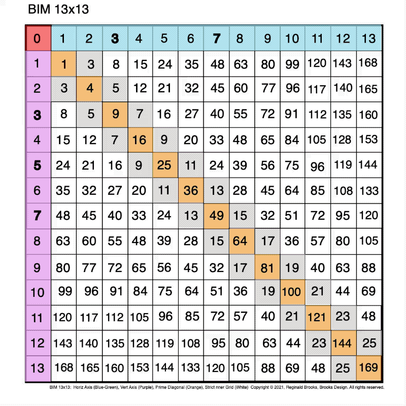

BIM-Goldbach_Conjecture, II (animated gif)

 

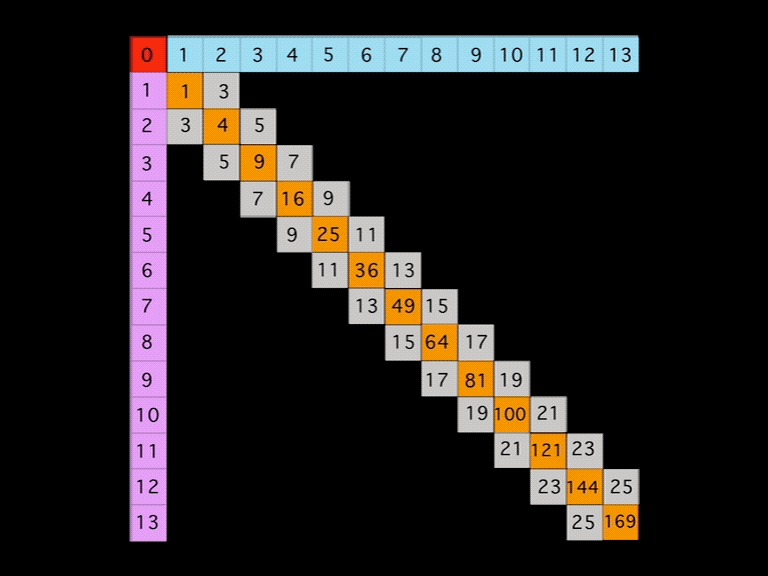
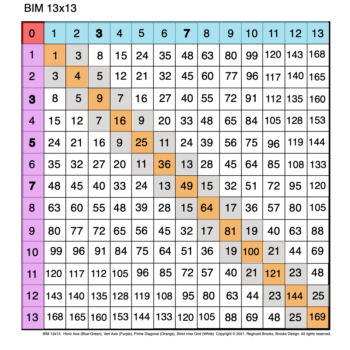Fig. 2.0 BIM-Goldbach_Conjecture, II-0. BIM grid.

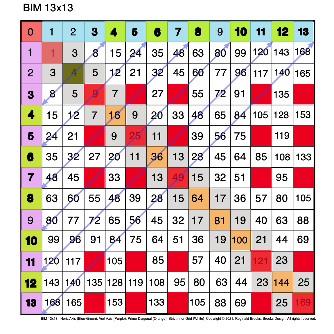Fig. 2.1 BIM-Goldbach_Conjecture, II-1. Diagonal lines between similar EVENS on the two Axis'. Red boxes are PPsets.

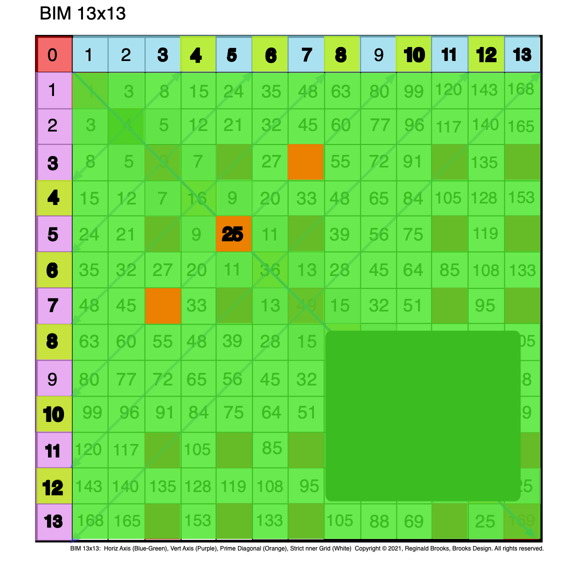Fig. 2.2 BIM-Goldbach_Conjecture, II-2. Green overlay to highlight Red PPsets.

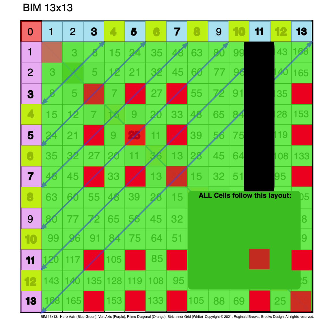Fig. 2.3 BIM-Goldbach_Conjecture, II-3. Green overlay to highlight Red PPsets + Diagonal lines between EVENS.

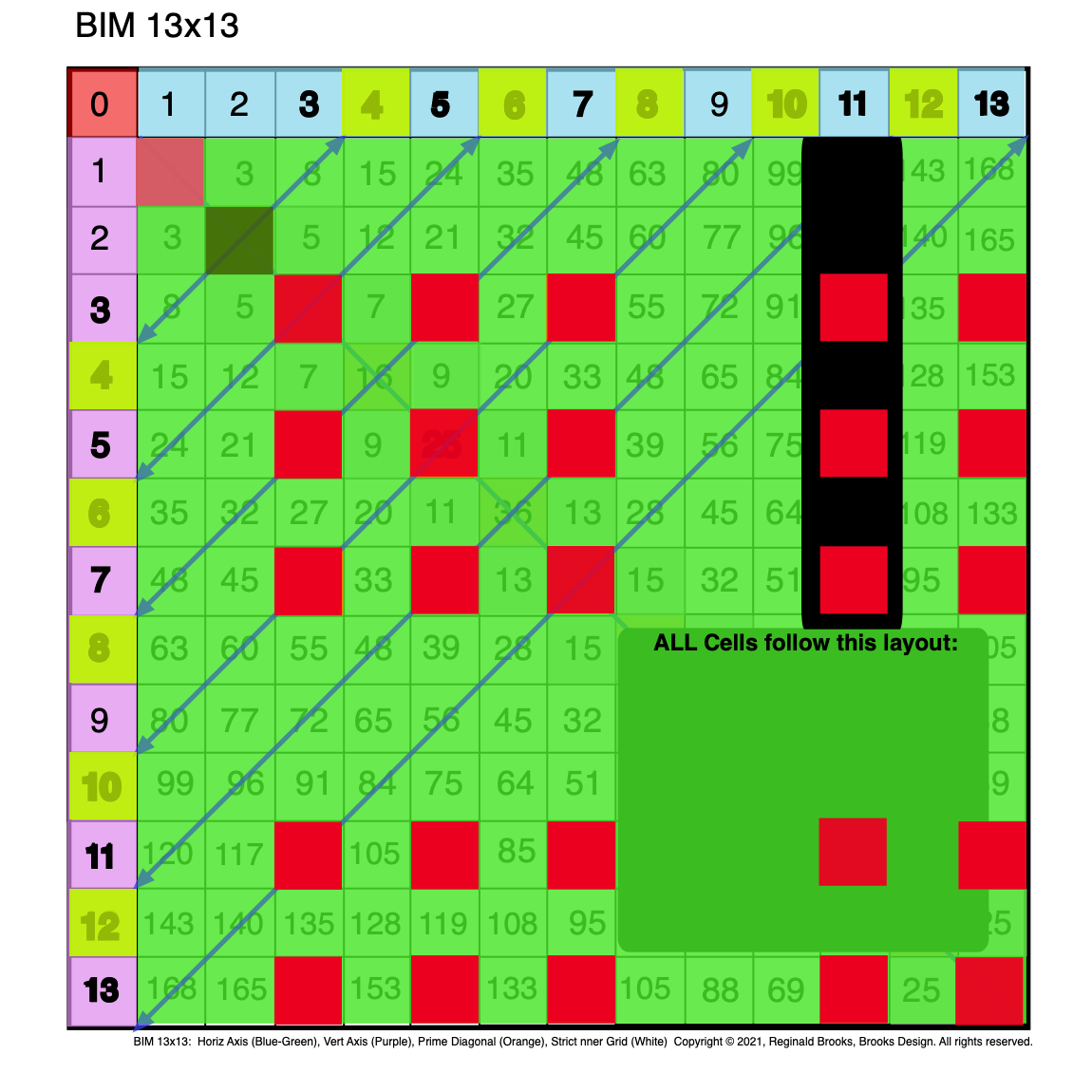Fig. 2.4 BIM-Goldbach_Conjecture, II-4. Green overlay to highlight Red PPsets + Diagonals + EVEN 4 (Dark Green) special case.

Fig. 2.5 BIM-Goldbach_Conjecture, II-5. Green overlay+Red PPsets+Diagonals + EVEN 4 (Dark Green)+EVEN 14 added.

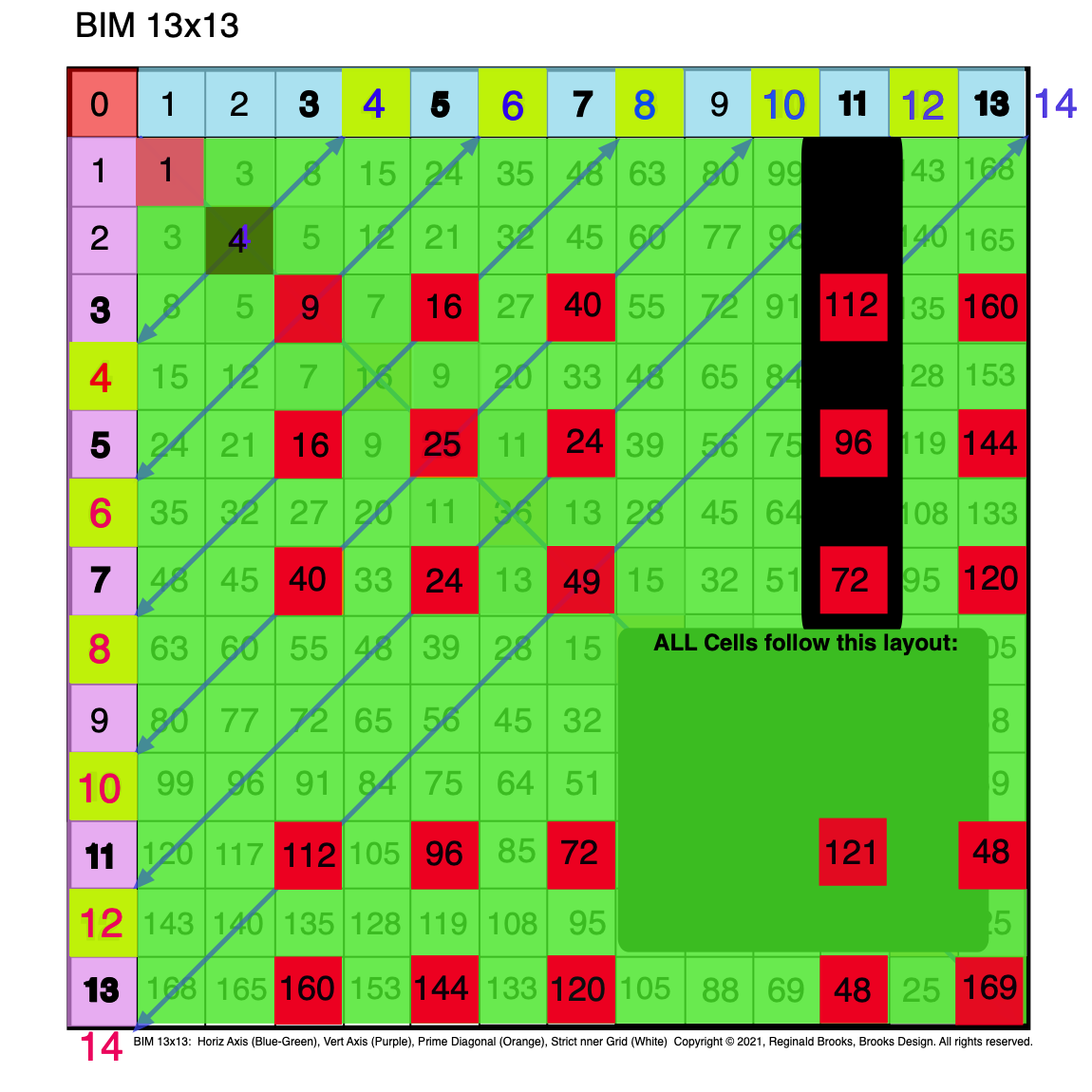Fig. 2.6 BIM-Goldbach_Conjecture, II-6. Green overlay+Red PPsets+Diagonals + EVEN 4+EVEN 14+ Cell Values added.

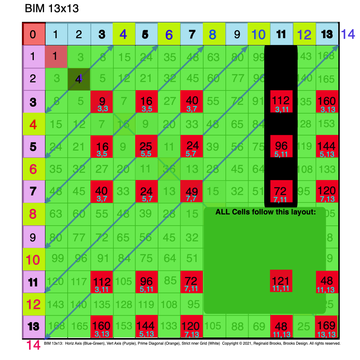Fig. 2.7 BIM-Goldbach_Conjecture, II-7. Axis Coordinate Values = PPsets (L.Blue-Green) added to BOTTOM of Cell Values.

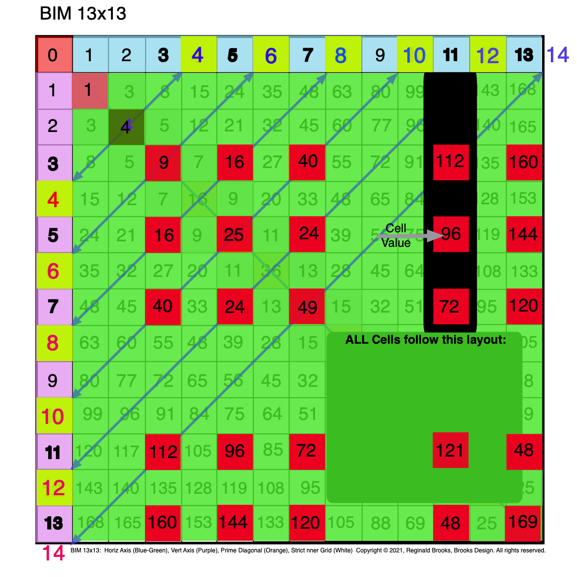Fig. 2.8 BIM-Goldbach_Conjecture, II-8. Re-emphisizing that the Cell Values (Black) are the large #s in the MIDDLE.

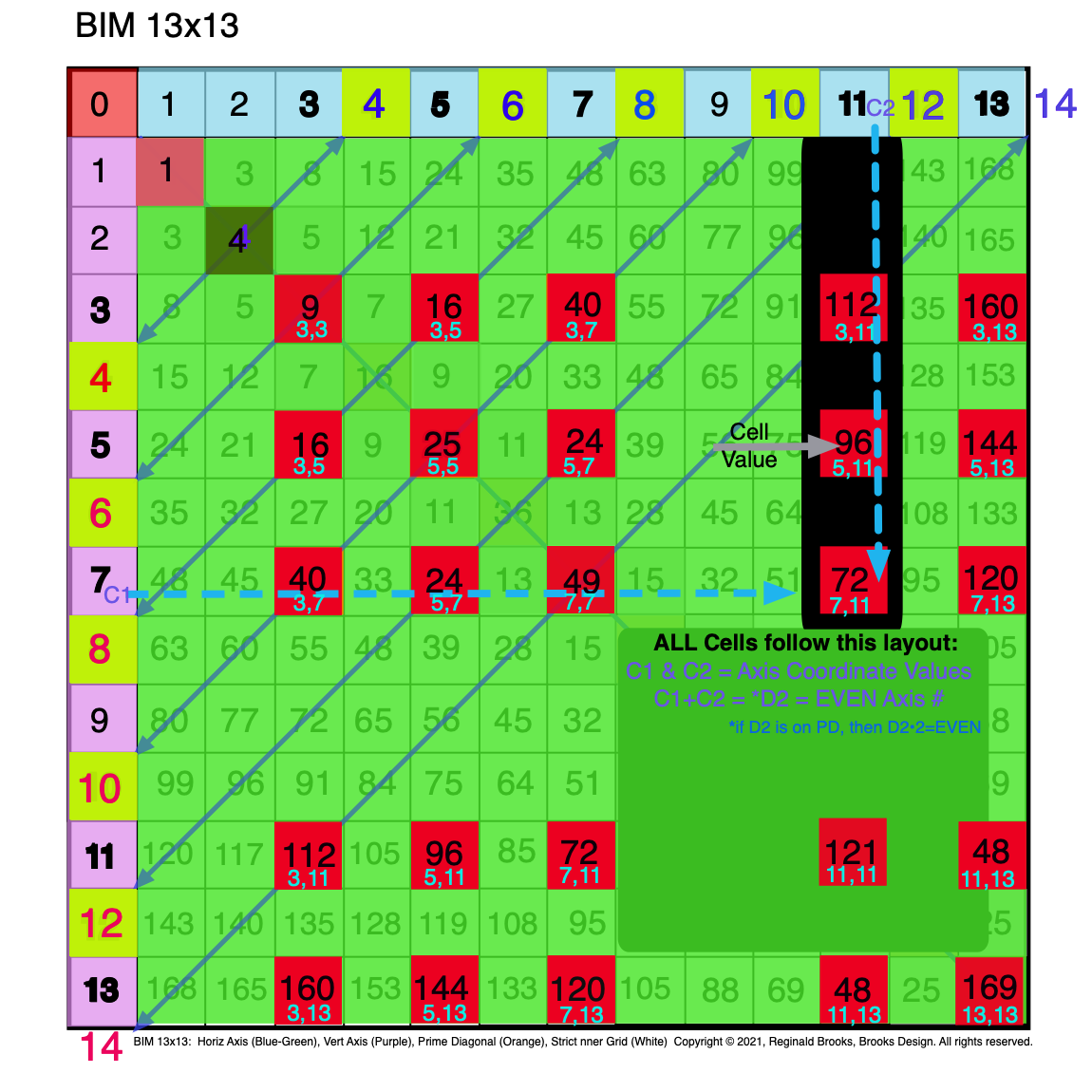Fig. 2.9 BIM-Goldbach_Conjecture, II-9. Axis Coordinate Values (C1,C2) = PPsets (L.Blue-Green) added to BOTTOM of Cell Values.

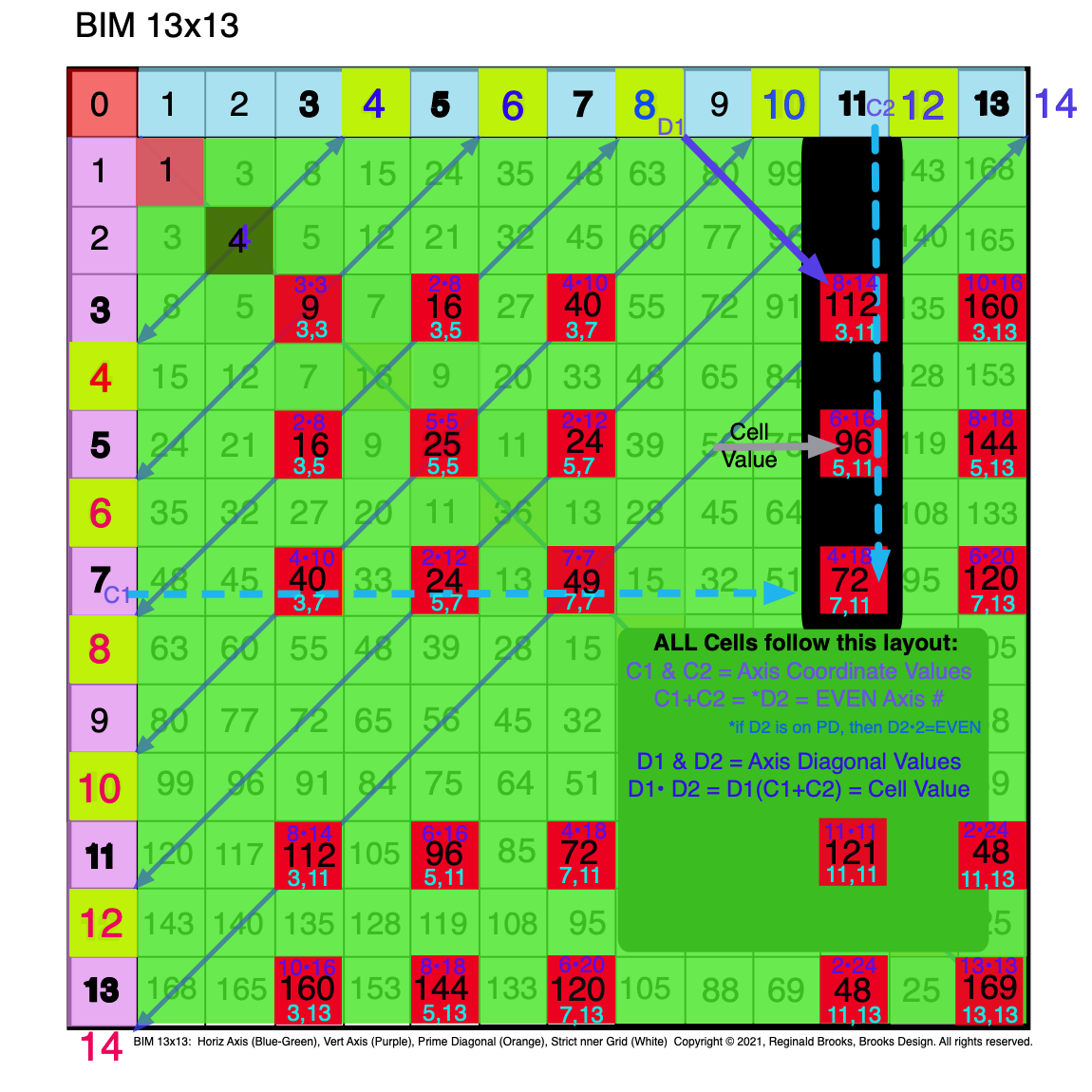Fig. 2.10 BIM-Goldbach_Conjecture, II-10. Axis Diagonal Values (D1•D2) = Cell Value (Dk.Blue) added to TOP of Cell Values.

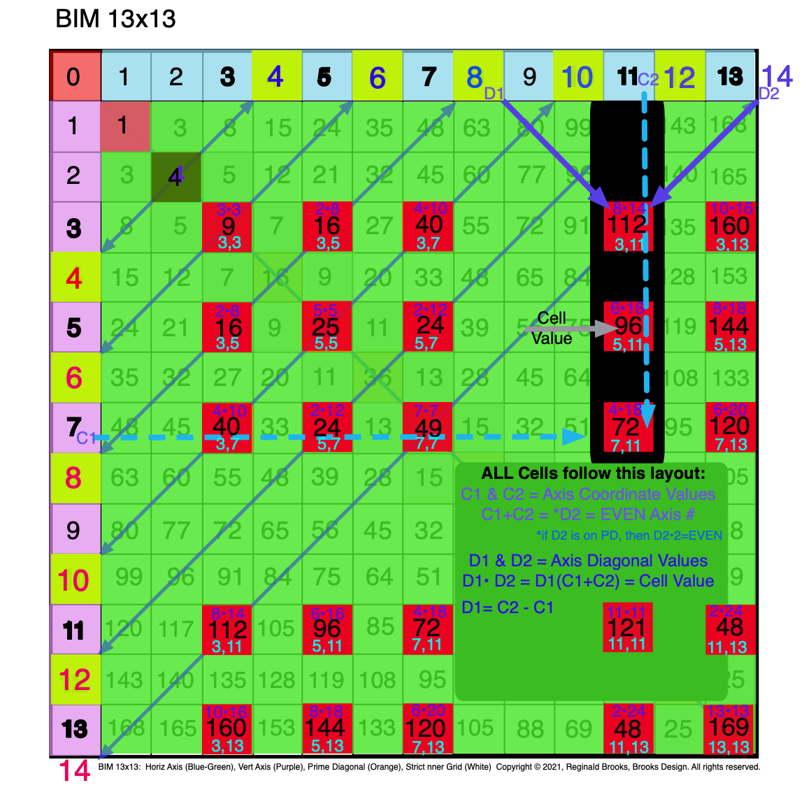Fig. 2.11 BIM-Goldbach_Conjecture, II-11. Axis Diagonal Values (D1•D2) = Cell Value (Dk.Blue) added to TOP of Cell Values.

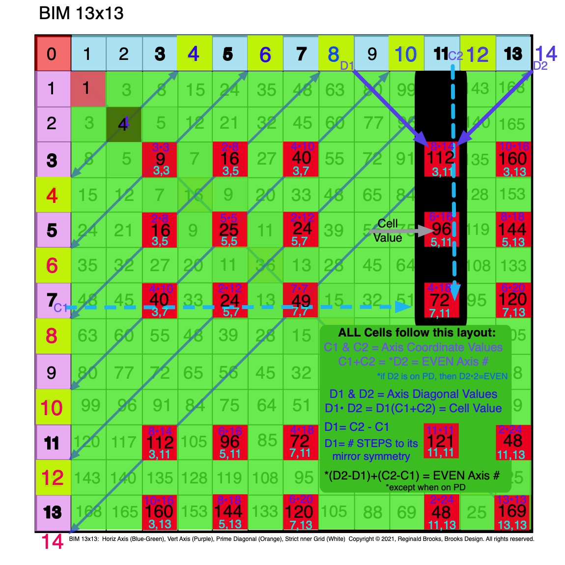Fig. 2.12 BIM-Goldbach_Conjecture, II-12. Axis Diagonal Values (D1•D2), Cell Values, and Axis Coordinate Values (C1,C2).

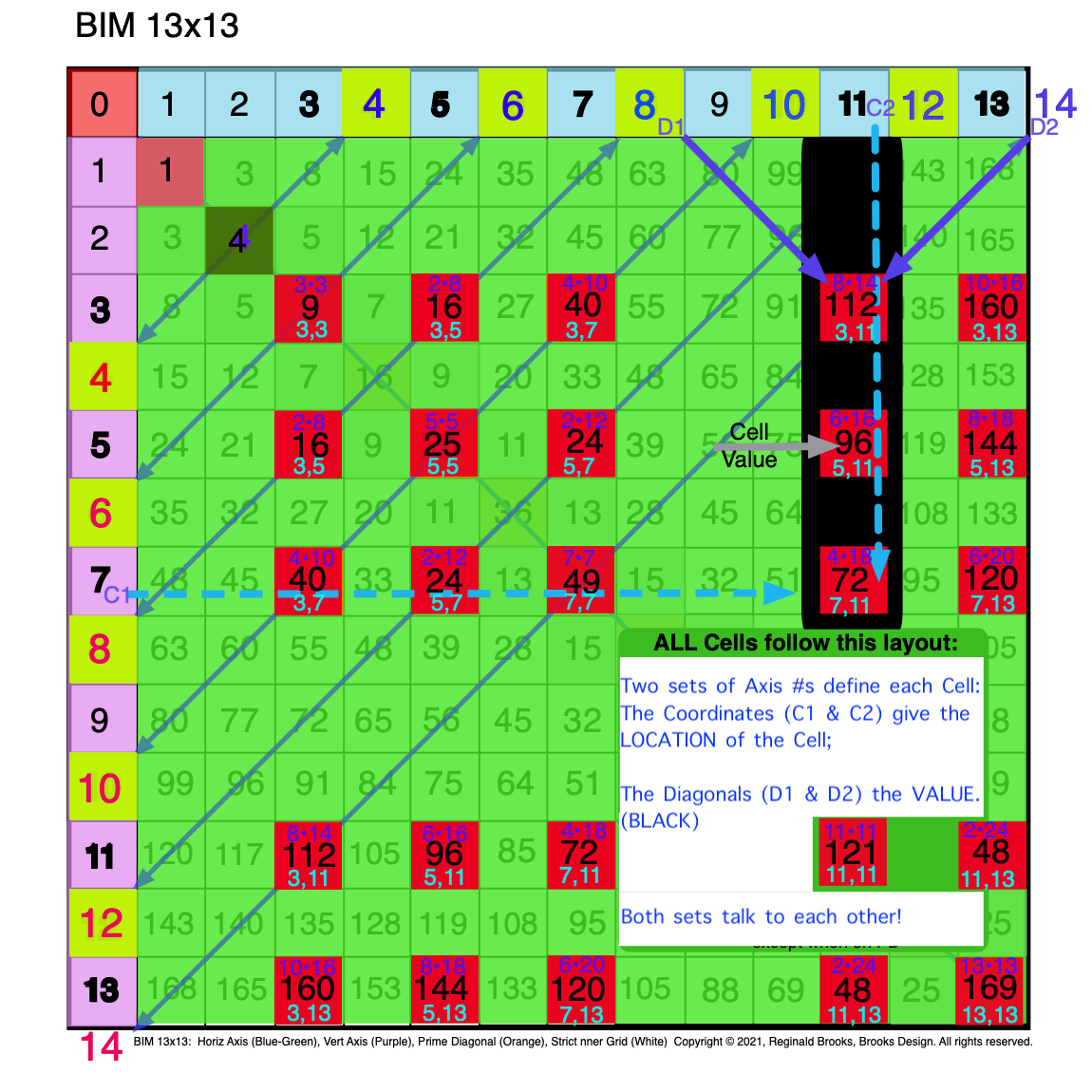Fig. 2.13 BIM-Goldbach_Conjecture, II-13. Axis Diagonal Values (D1•D2) and Axis Coordinate Values (C1,C2) define Cell Values.

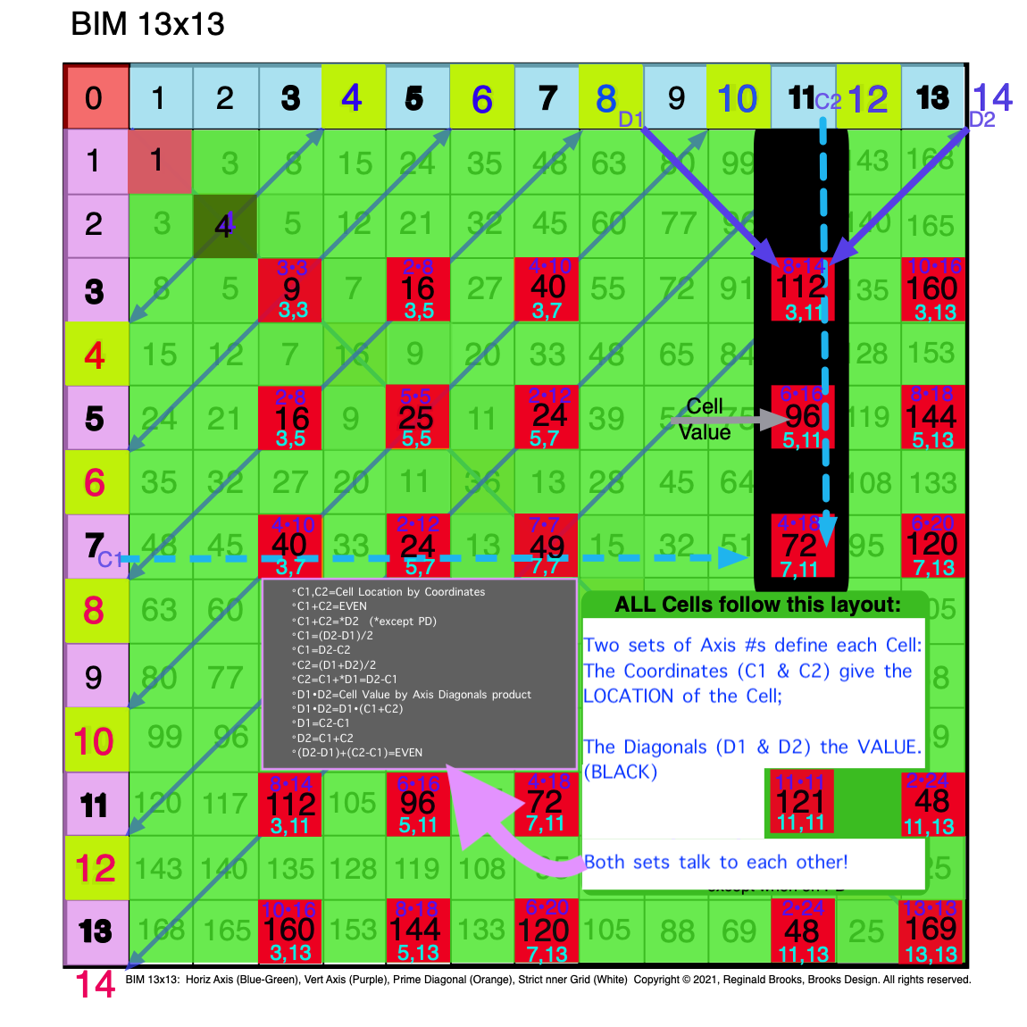Fig. 2.14 BIM-Goldbach_Conjecture, II-14. Axis Diagonal Values (D1•D2) and Axis Coordinate Values (C1,C2) define Cell Values.

 

Summary

In Part II, we have had a further simplification! Though at first glance it may seem more complicated, it really is not once you realize that every cell in the BIM follows this same pattern. Each grid cell is defined by two sets of Axis numbers:

 

1. The Axis Coordinates (C1 & C2)— one on the Top horizontal Axis and one on the Left vertical Axis — provide the grid cell LOCATION. They are found on the BOTTOM of the Cell grid;
2. The Axis Diagonals (D1 & D2)— both values from either the Top horizontal or the Left-side vertical Axis — diagonally converge on a grid cell VALUE. They are found on the TOP of the Cell grid.

 

Together, these two sets of values provide information about that respective grid cell value, inter-relate to each other, and inform — when in Diagonal line — the value of the related EVEN number they are connected with!

 

Here is a SUMMARY:

 

◦C1,C2=Cell Location by Coordinates

◦C1+C2=EVEN

◦C1+C2=D2 (except PD)

◦C1=(D2-D1)/2

◦C1=D2-C2

◦C2=(D1+D2)/2

◦C2=C1+*D1=D2-C1

◦D1•D2=Cell Value by Axis Diagonals product

◦D1•D2=D1•(C1+C2)

◦D1=C2-C1

◦D2=C1+C2

◦(D2-D1)+(C2-C1)=EVEN

 

 

3. Shape

Shape: Each of the above 3 parameters can be easily shown to be the apex value of three Right-Isosceles Triangles providing a very natural, intuitive depiction of the relationship of the parameters to each grid cell.

Video

BIM-Goldbach_Conjecture_III from Reginald Brooks on Vimeo.

Images

BIM-Goldbach_Conjecture, III (animated gif)

 

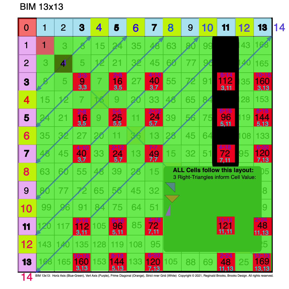Fig. 3.1 BIM-Goldbach_Conjecture, III-1. Three (3) Right-Triangles inform the Cell Values.

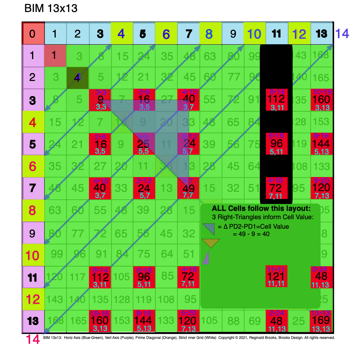Fig. 3.2 BIM-Goldbach_Conjecture, III-2. The BlueGreen R-Isosceles Triangle = Difference (∆) between PD2-PD1=Cell Value.

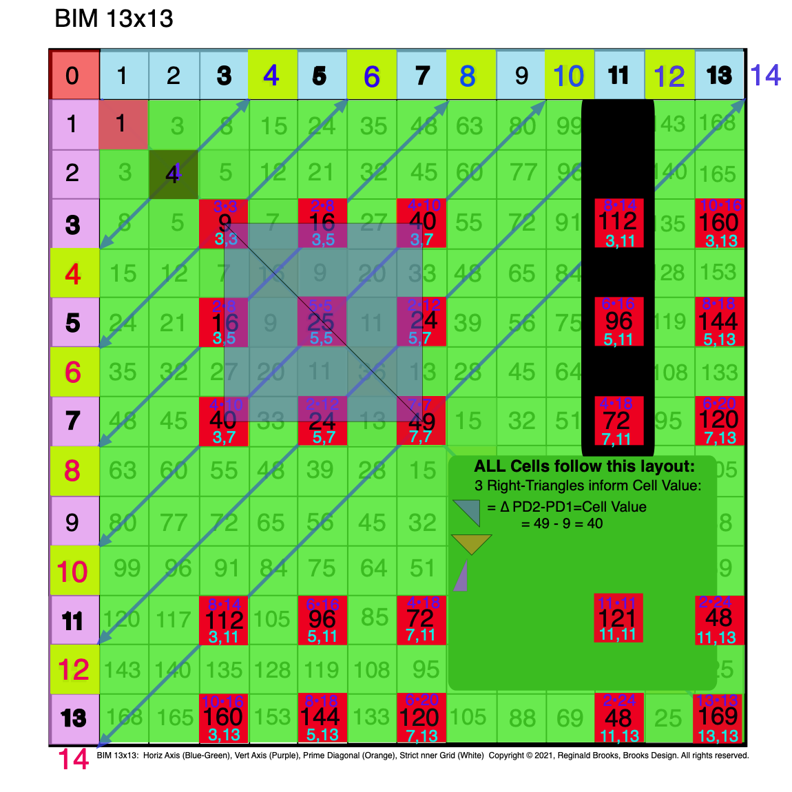Fig. 3.3 BIM-Goldbach_Conjecture, III-3. Symmetry: The BG R-Isosceles Triangle = Difference (∆) between PD2-PD1=Cell Value.

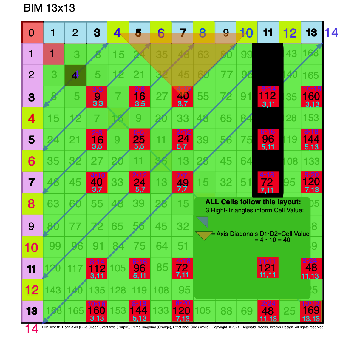Fig. 3.4 BIM-Goldbach_Conjecture, III-4. The Orange R-Isosceles Triangle = D1 • D2 = Cell Value.

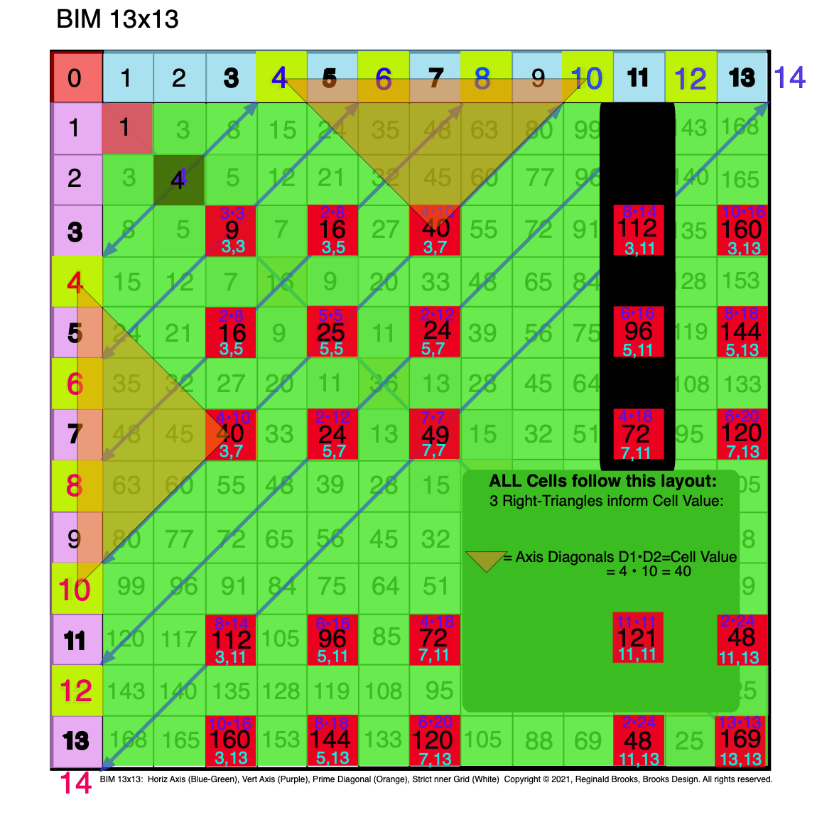Fig. 3.5 BIM-Goldbach_Conjecture, III-5. Symmetry: The Orange R-Isosceles Triangle = D1 • D2 = Cell Value.

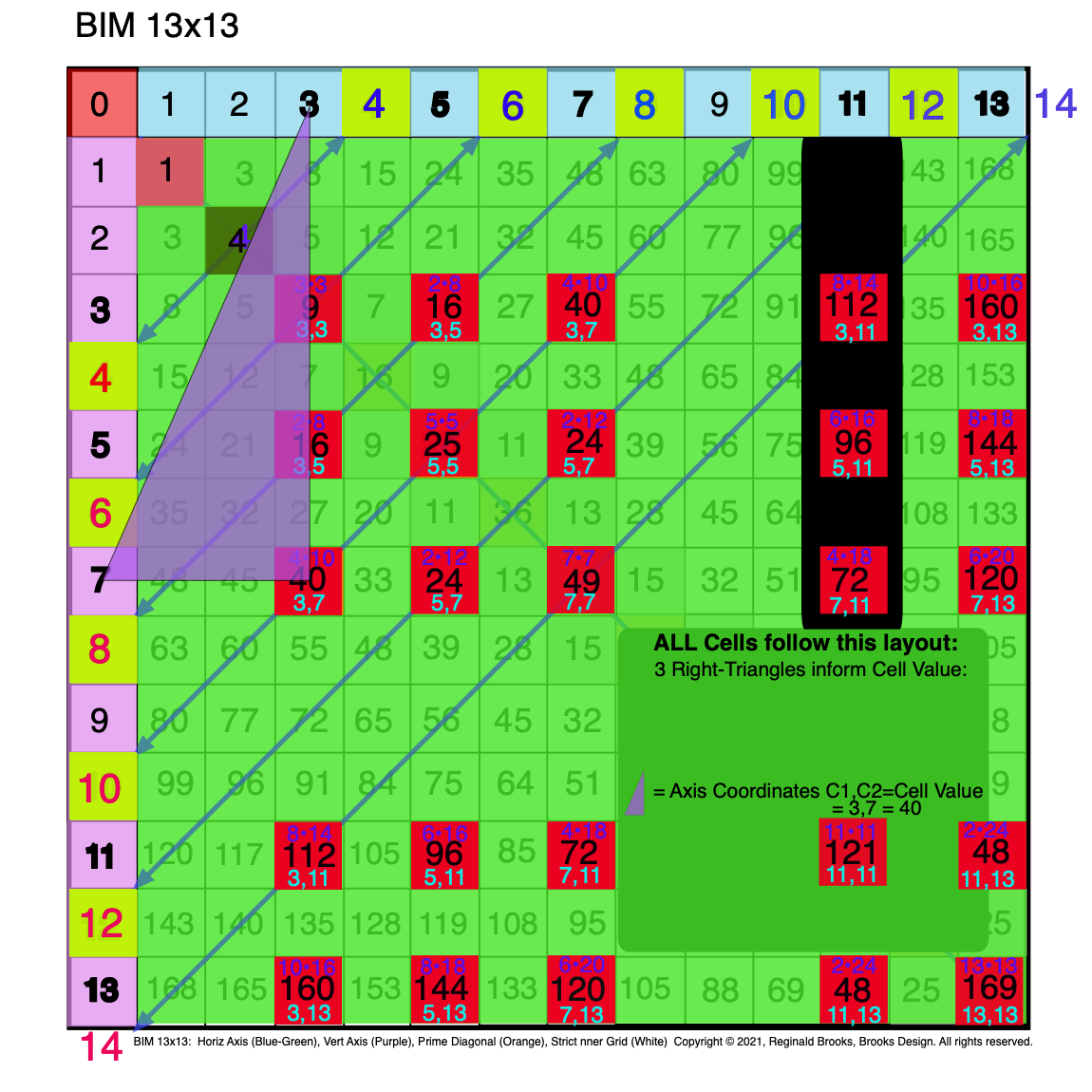Fig. 3.6 BIM-Goldbach_Conjecture, III-6. The Purple R-Triangle = C1, C2 = Cell Value Location = PPset.

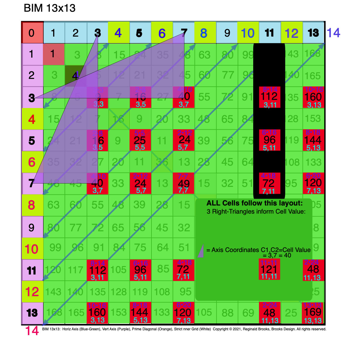Fig. 3.7 BIM-Goldbach_Conjecture, III-7. Symmetry: The Purple R-Triangle = C1, C2 = Cell Value Location = PPset.

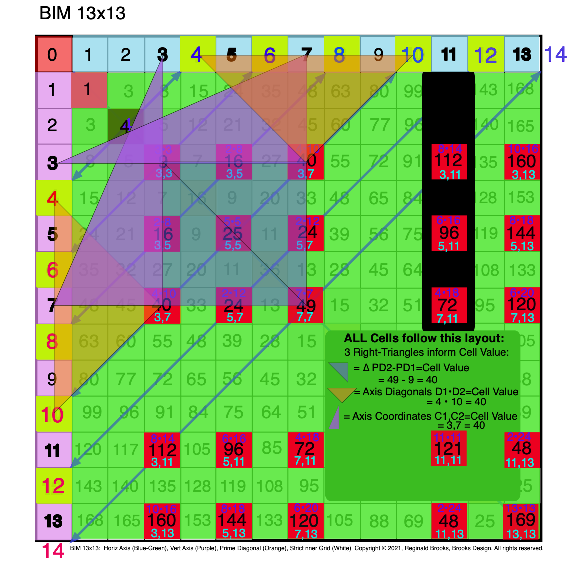Fig. 3.8 BIM-Goldbach_Conjecture, III-8. Symmetry: The Purple R-Triangle & Orange R-Isosceles & BG R-Isosceles Triangles.

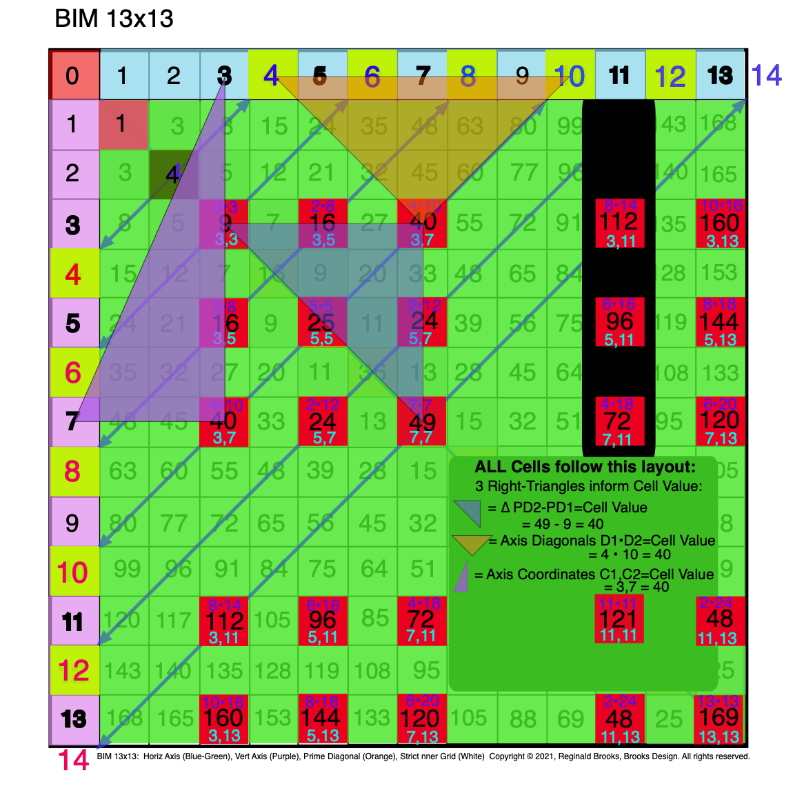Fig. 3.9 BIM-Goldbach_Conjecture, III-9. The Purple R-Triangle & Orange R-Isosceles & BG R-Isosceles Triangles.

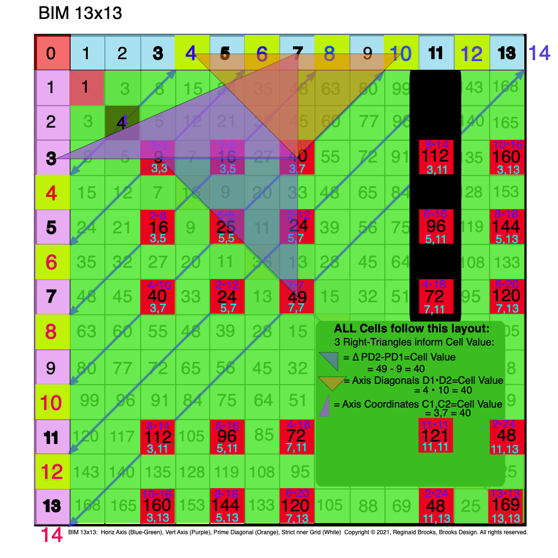Fig. 3.10 BIM-Goldbach_Conjecture, III-10. The Purple R-Triangle & Orange R-Isosceles & BG R-Isosceles Triangles.

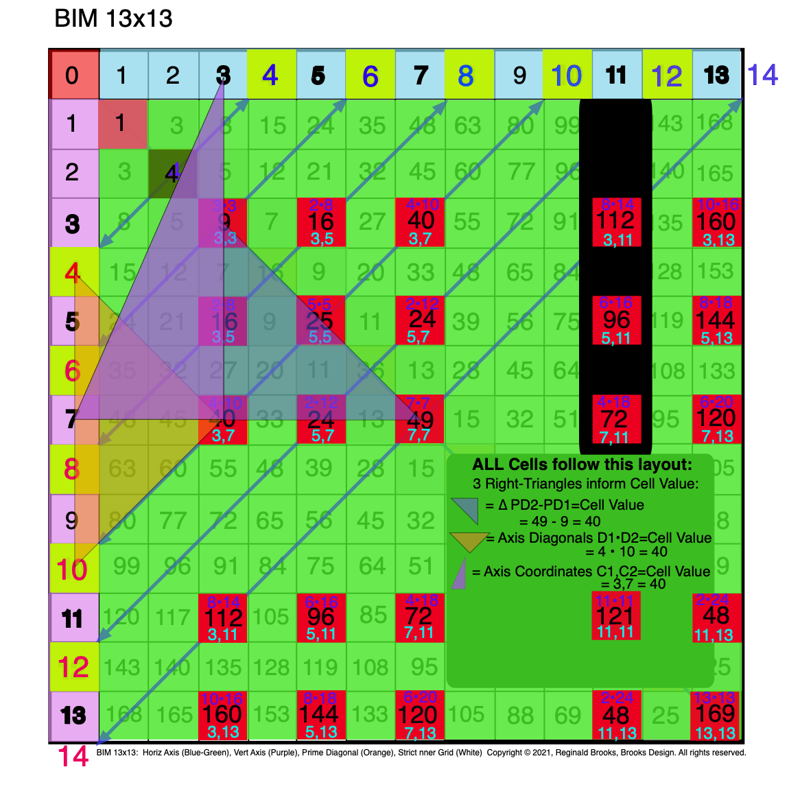Fig. 3.11 BIM-Goldbach_Conjecture, III-11. The Purple R-Triangle & Orange R-Isosceles & BG R-Isosceles Triangles.

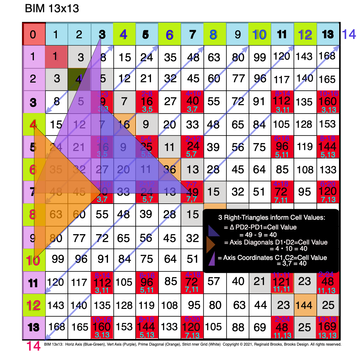Fig. 3.12 BIM-Goldbach_Conjecture, III-12. The Purple R-Triangle & Orange R-Isosceles & BG R-Isosceles Triangles.

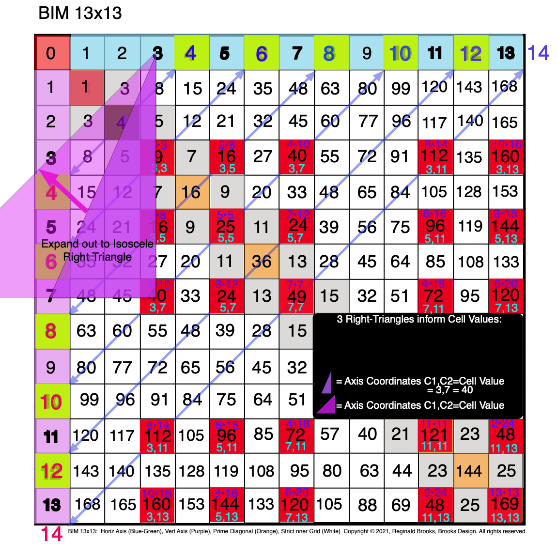Fig. 3.13 BIM-Goldbach_Conjecture, III-13. The C1,C2 Purple R-Triangle expanded out to make an R-Isosceles Triangle.

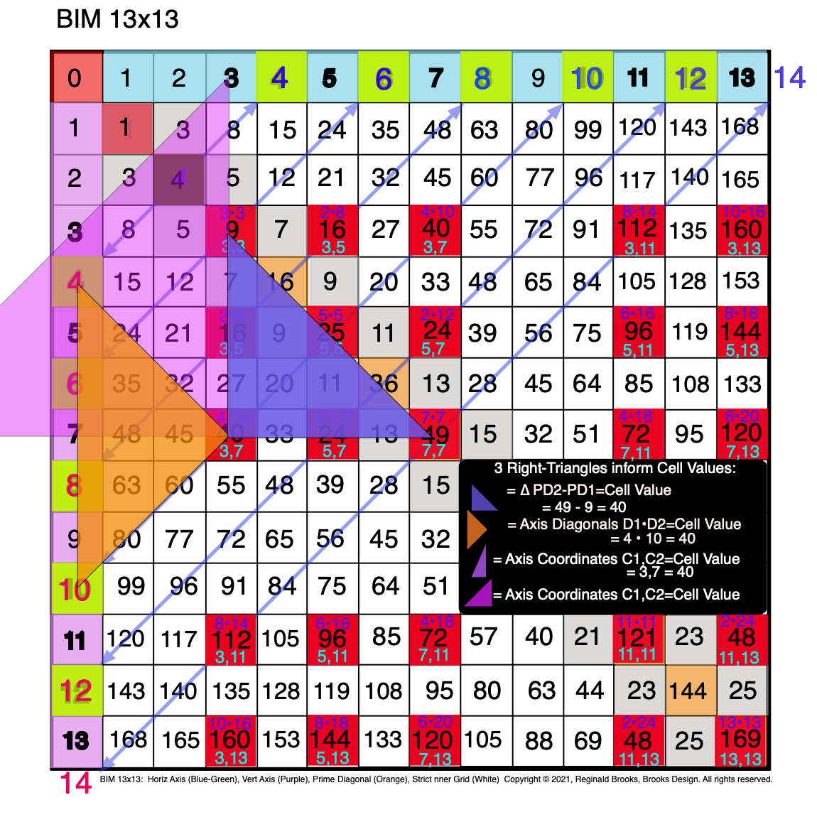Fig. 3.14 BIM-Goldbach_Conjecture, III-14. All three R-Triangles are now shown as R-Isosceles Triangles.

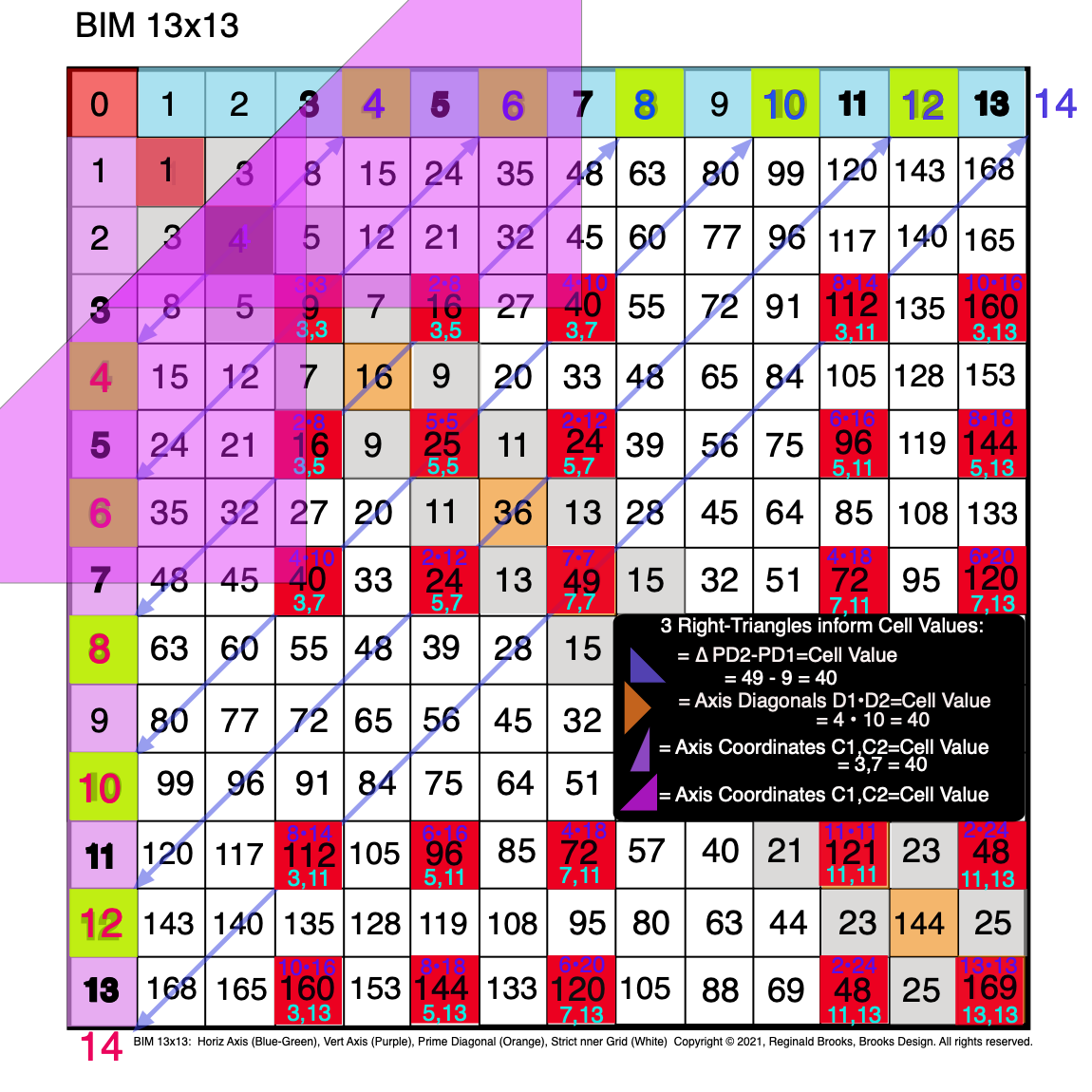Fig. 3.15 BIM-Goldbach_Conjecture, III-15. Symmetry: The Axis Coordinates (C1,C2) as R-Isosceles Triangles (truncated).

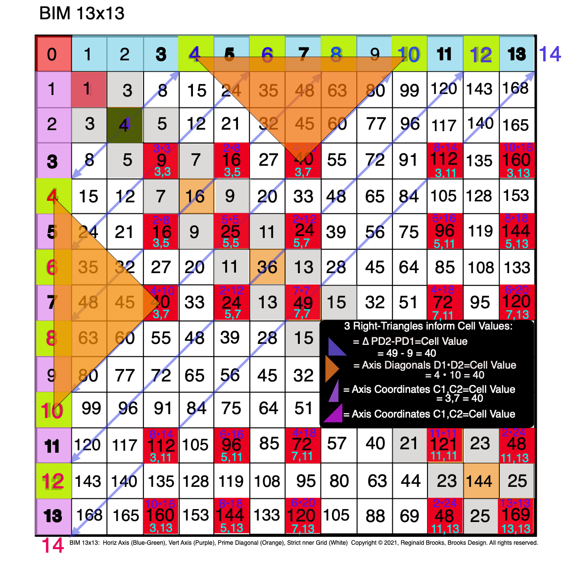Fig. 3.16 BIM-Goldbach_Conjecture, III-16. Symmetry: The Orange R-Isosceles Triangle = D1 • D2 = Cell Value.

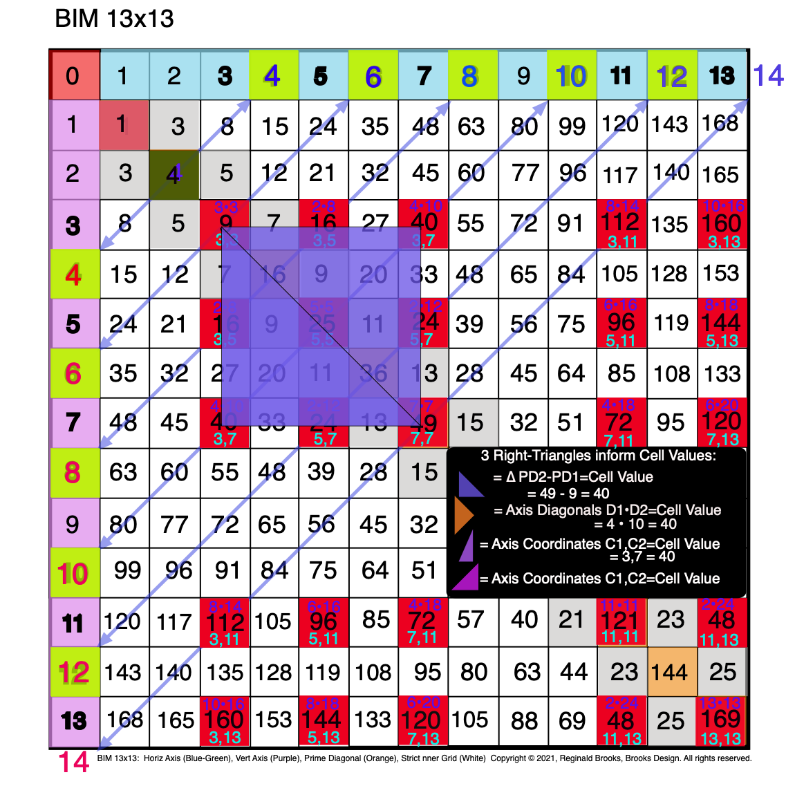Fig. 3.17 BIM-Goldbach_Conjecture, III-17. Symmetry: The Blue R-Isosceles Triangle =∆ between PD2-PD1=Cell Values.

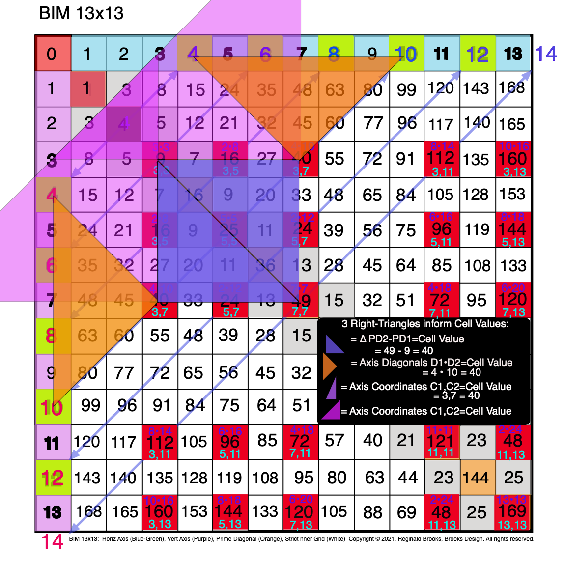Fig. 3.18 BIM-Goldbach_Conjecture, III-18. Symmetry: All three R-Triangles are now shown as R-Isosceles Triangles.

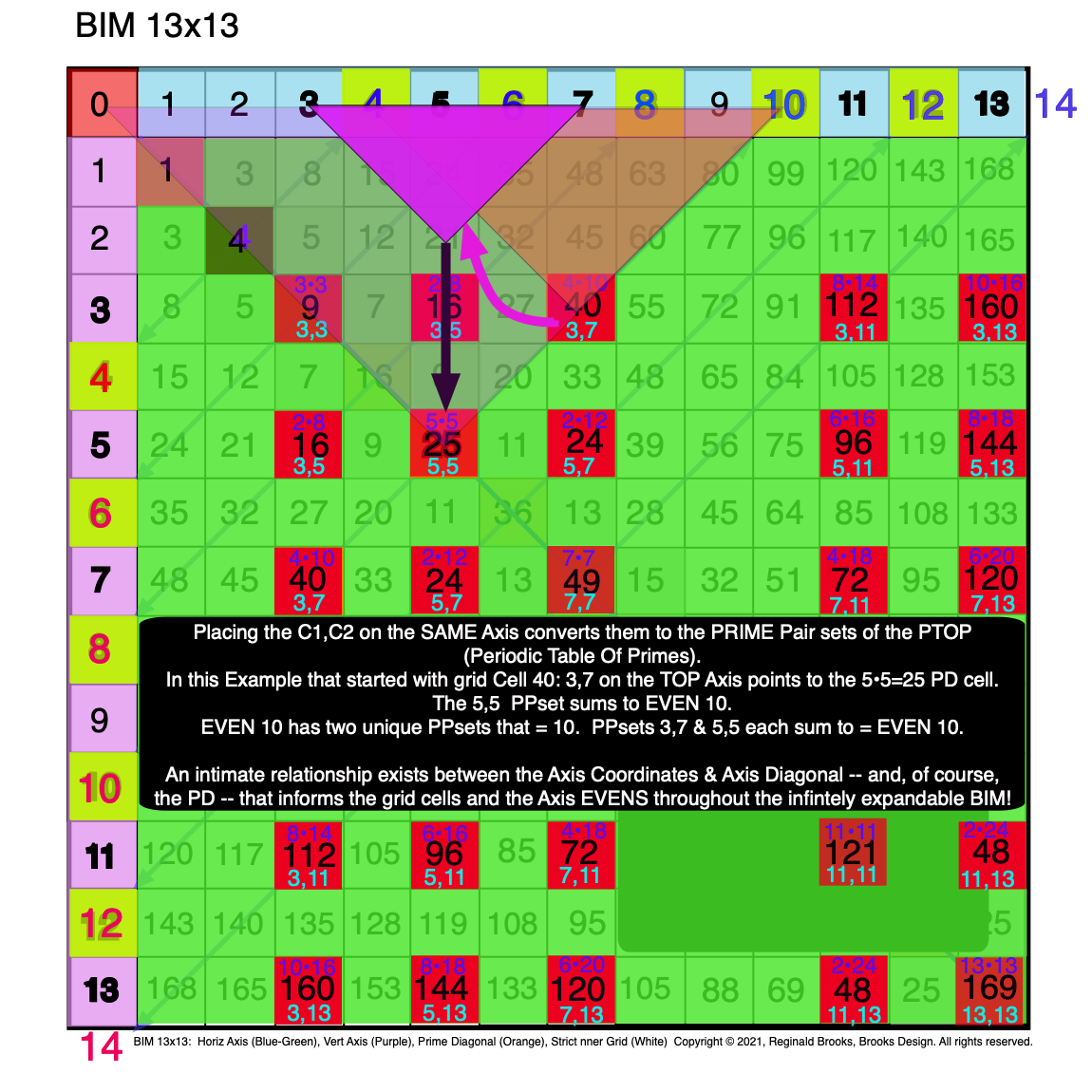Fig. 3.19 BIM-Goldbach_Conjecture, III-19. All three R-Triangles are now shown as R-Isosceles Triangles in a new configuration.

 

Summary

In Part III, we have had a further simplification: Right-Isosceles Triangles!

 

In Part II we wrote: Though at first glance it may seem more complicated, it really is not once you realize that every cell in the BIM follows this same pattern. Each grid cell is defined by two sets of Axis numbers:

 

1. The Axis Coordinates (C1 & C2)— one on the Top horizontal Axis and one on the Left vertical Axis — provide the grid cell LOCATION;

2. The Axis Diagonals (D1 & D2)— both values from either the Top horizontal or the Left-side vertical Axis — diagonally converge on a grid cell VALUE.

   Actually, if one considers just the Inner Grid (IG) cells, a third parameter:

3. The difference in the Prime Diagonals (PD2 - PD1) — from the Row & Column intersect — provide the grid cell VALUE, too.

 

All 3 of the above parameters can be represented by a Right-angled Isosceles Triangle.

 

Part III presents examples of a number of grid cells that intersect with the Axis EVEN #s via a Diagonal between the two Axis’. We do so with the 3 parameters defining said grid cell defined by their 3 colored R-Isosceles Triangles.

 

 

4. Integration

Integration: Combining all, or just key parts, of the individual lines, layout parameters and shapes reveals how ultimately every PPset is interconnected and also ultimately how the PRIMES, the building blocks of all the "other" numbers, are themselves interconnected, symmetry based fractal-configured relationships between simple notions of quantity as expressed by numerical symbols.

 

Video

BIM-Goldbach_Conjecture_IV from Reginald Brooks on Vimeo.

Images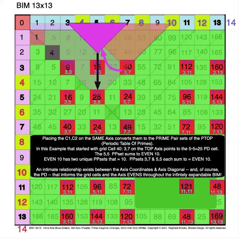

BIM-Goldbach_Conjecture, IV (animated gif)

 

Fig. 4.1 BIM-Goldbach_Conjecture, IV-1. All three R-Triangles are now shown as R-Isosceles Triangles in a new configuration.

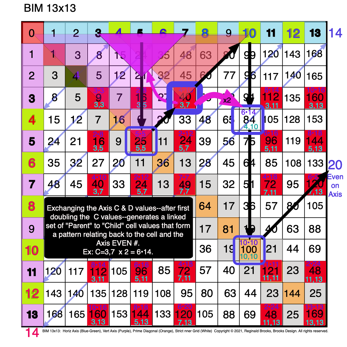Fig. 4.2 BIM-Goldbach_Conjecture, IV-2. Exchanging D & double C values links the "Parent" Cell to one of its "Child" Cells.

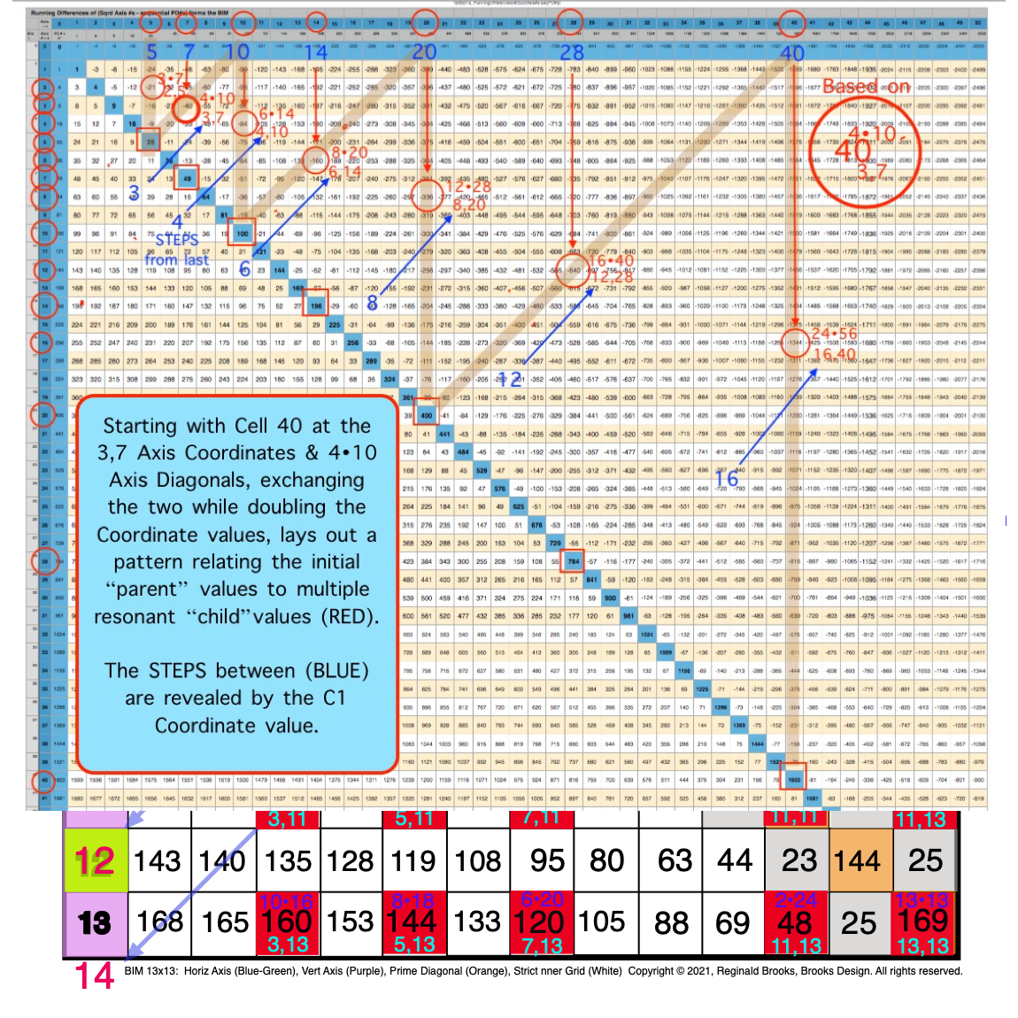Fig. 4.3 BIM-Goldbach_Conjecture, IV-3. The "Parent" Cell to one, or more, of its "Child" Cells forms a regular pattern.

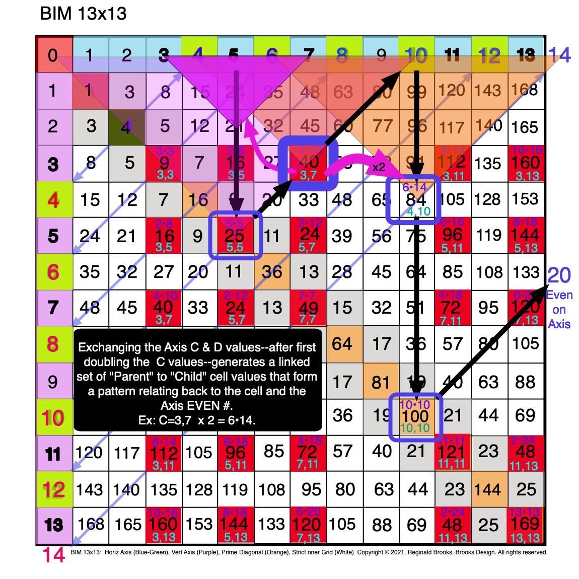Fig. 4.4 BIM-Goldbach_Conjecture, IV-4. The "Child" Cell relates back, via its Axis Diagonal Triangle to the "Parent's" PD2 value.

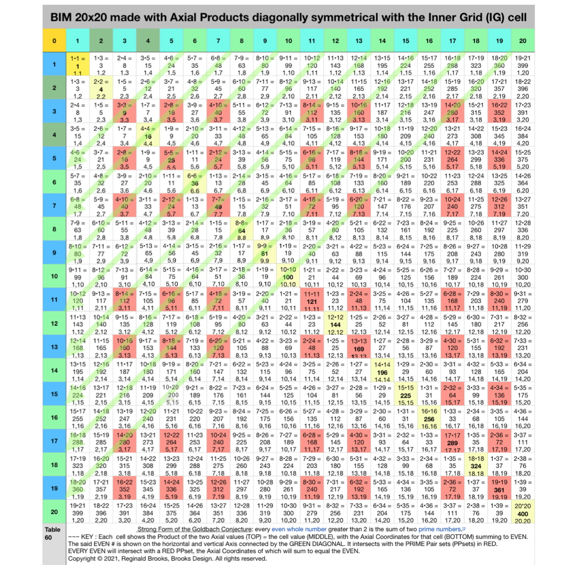Fig. 4.5 BIM-Goldbach_Conjecture, IV-5. Larger BIM20x20 with Red PPset Squares intersected by Green Diagonals from EVENS.

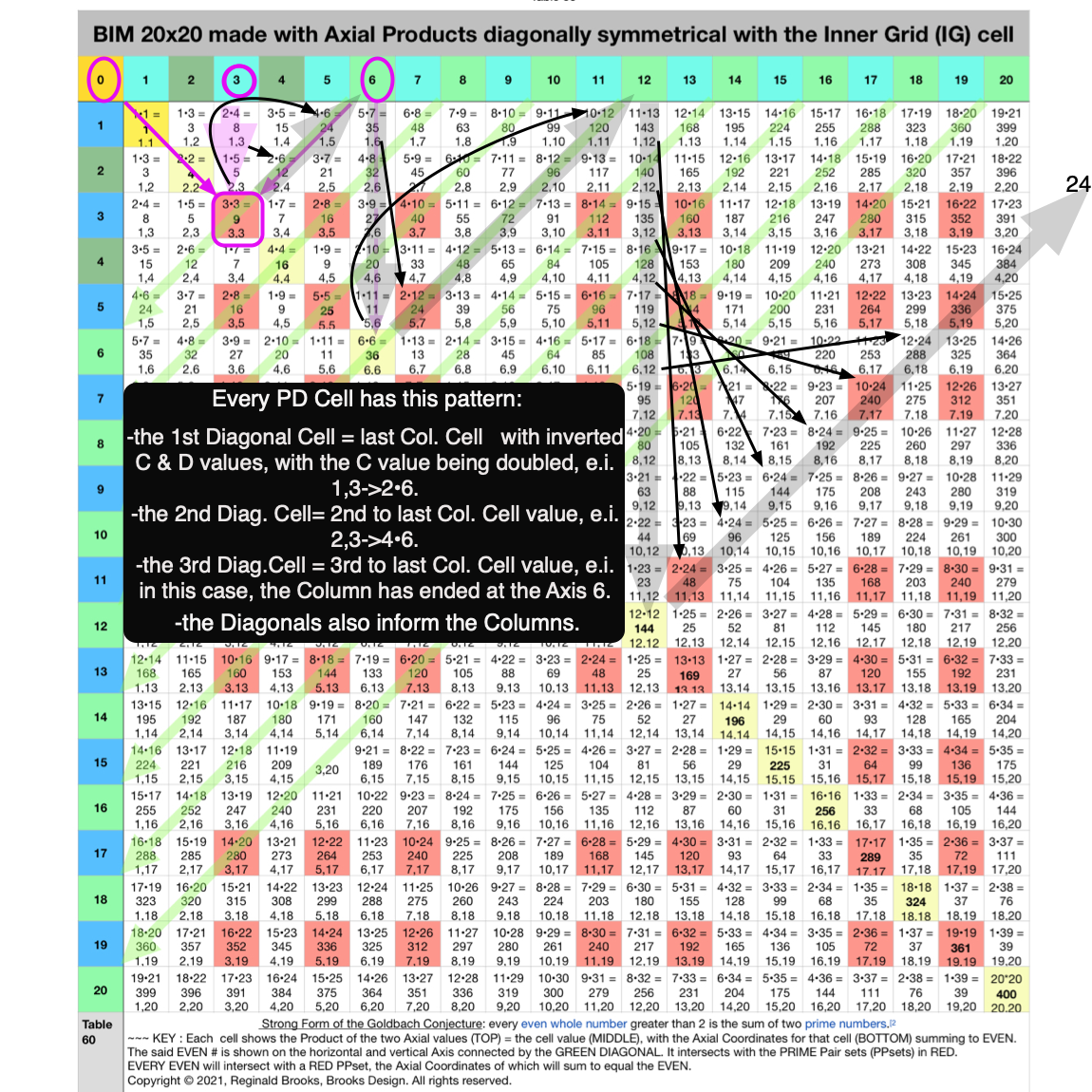Fig. 4.6 BIM-Goldbach_Conjecture, IV-6. The "Parent" Cell to one, or more, of its "Child" Cells forms a regular DIAGONAL pattern.

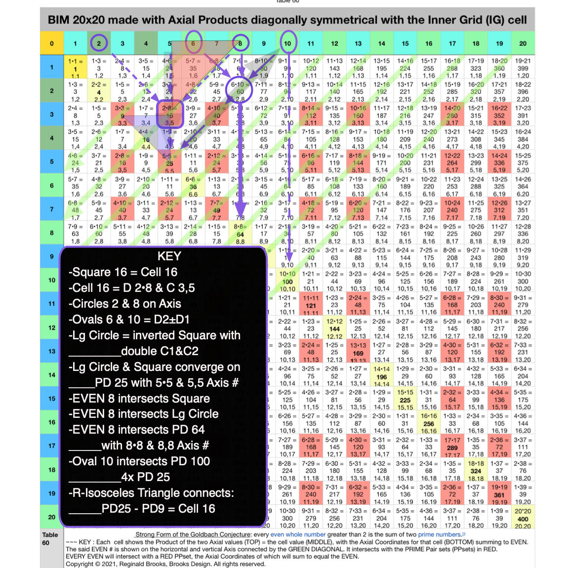Fig. 4.7 BIM-Goldbach_Conjecture, IV-7. Square 16 LINE, LAYOUT & SHAPE Cell pattern.

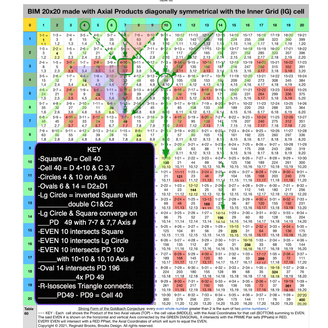Fig. 4.8 BIM-Goldbach_Conjecture, IV-8. Square 40 LINE, LAYOUT & SHAPE Cell pattern.

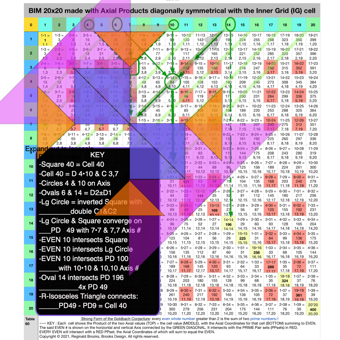Fig. 4.9 BIM-Goldbach_Conjecture, IV-9. Playing with spinning the 3-R-Isosceles Triangles around the 49.

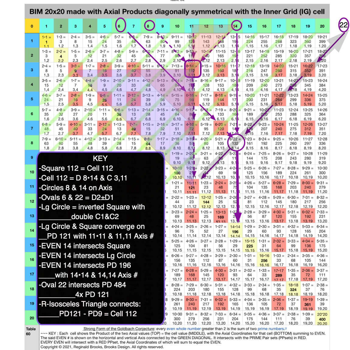Fig. 4.10 BIM-Goldbach_Conjecture, IV-10. Square 112 LINE, LAYOUT & SHAPE Cell pattern.

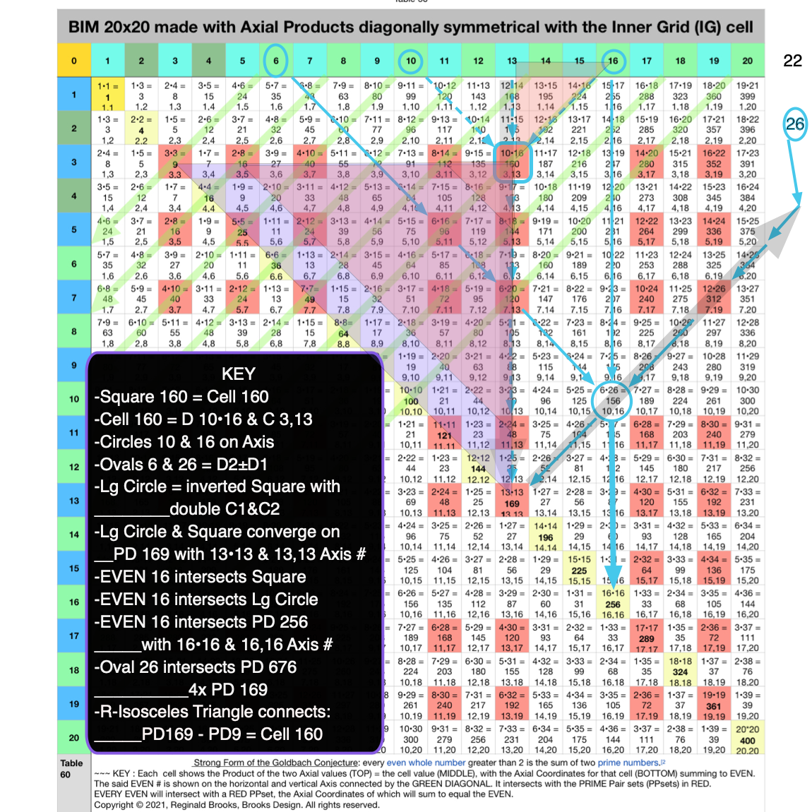Fig. 4.11 BIM-Goldbach_Conjecture, IV-11. Square 160 LINE, LAYOUT & SHAPE Cell pattern.

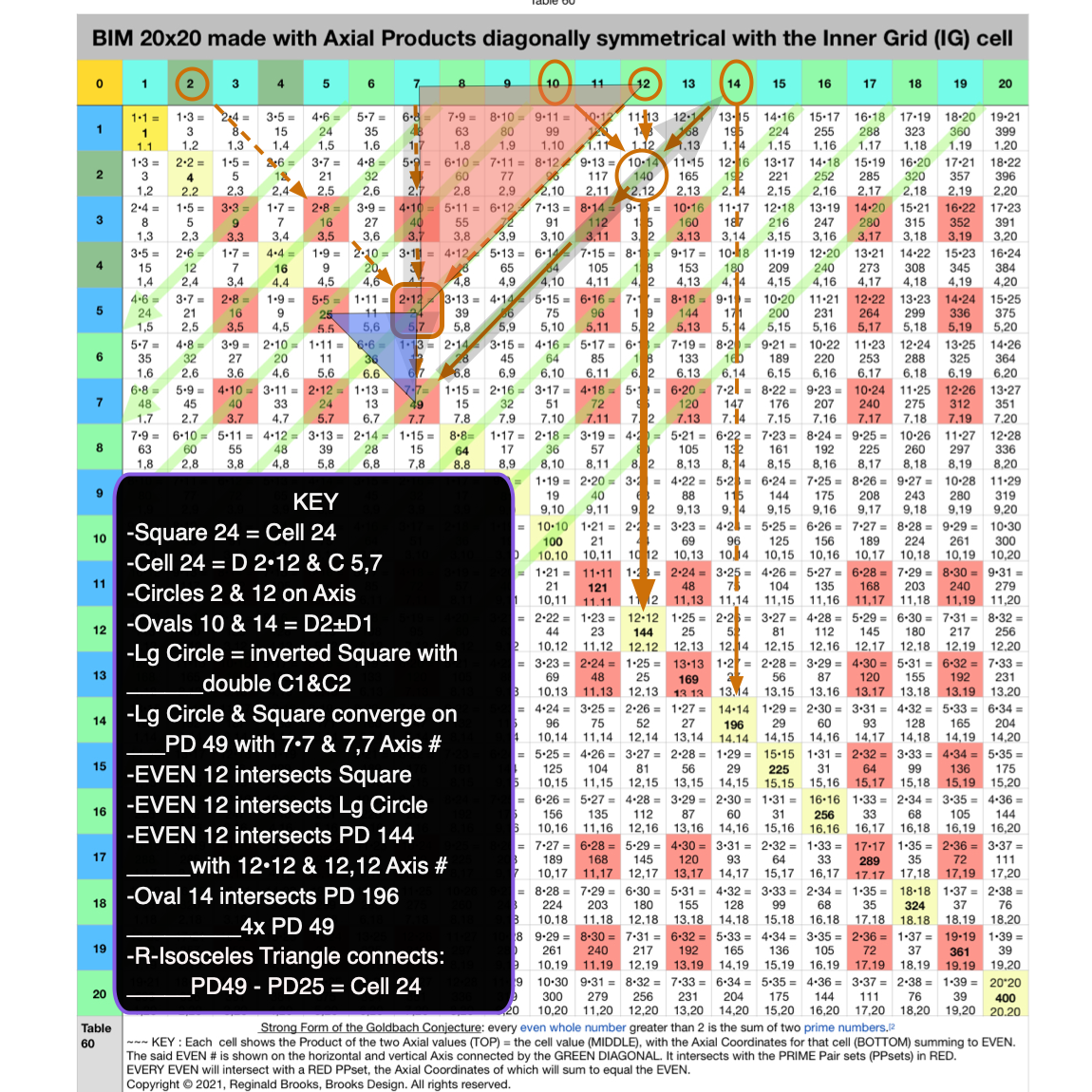Fig. 4.12 BIM-Goldbach_Conjecture, IV-12. Square 24 LINE, LAYOUT & SHAPE Cell pattern.

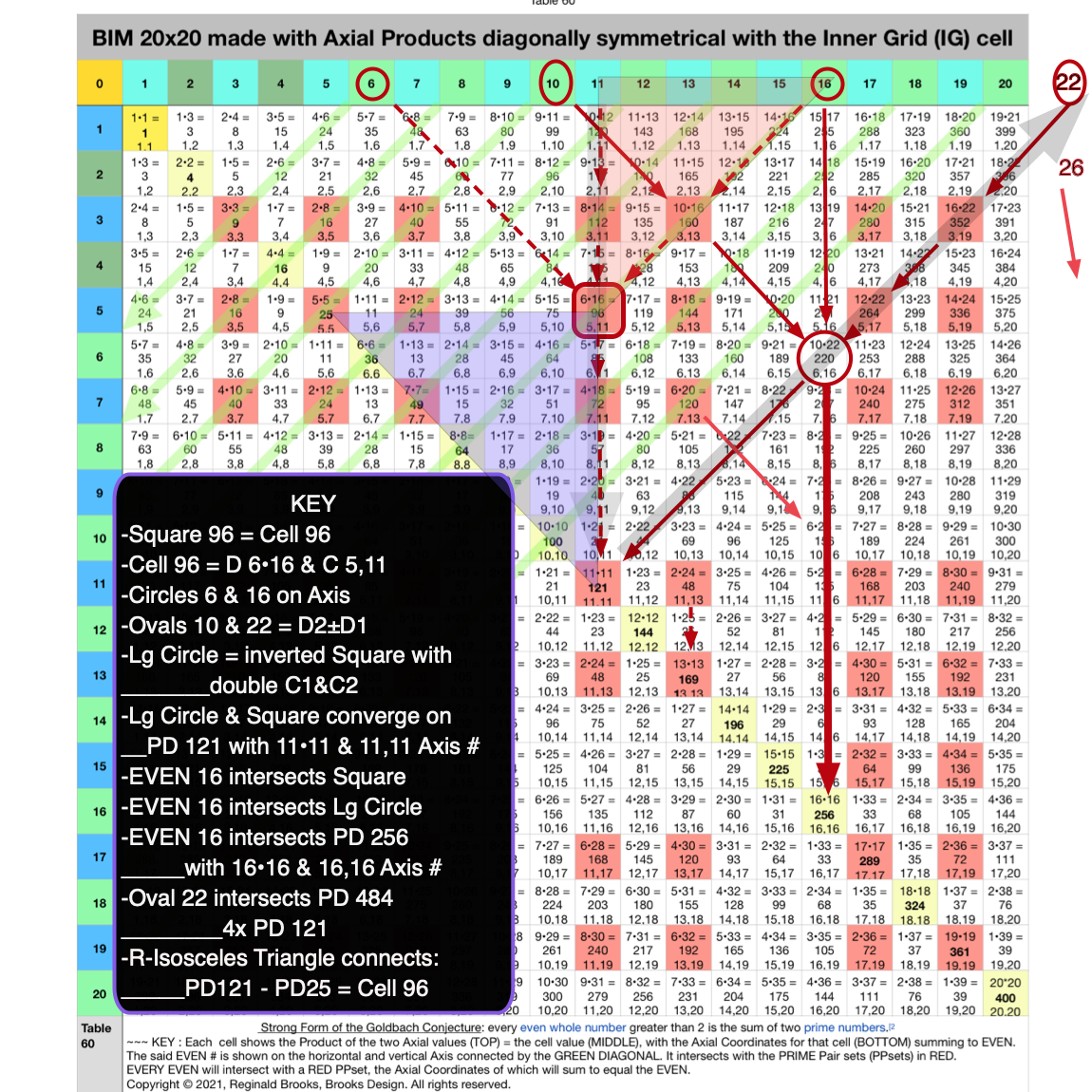Fig. 4.13 BIM-Goldbach_Conjecture, IV-13. Square 96 LINE, LAYOUT & SHAPE Cell pattern.

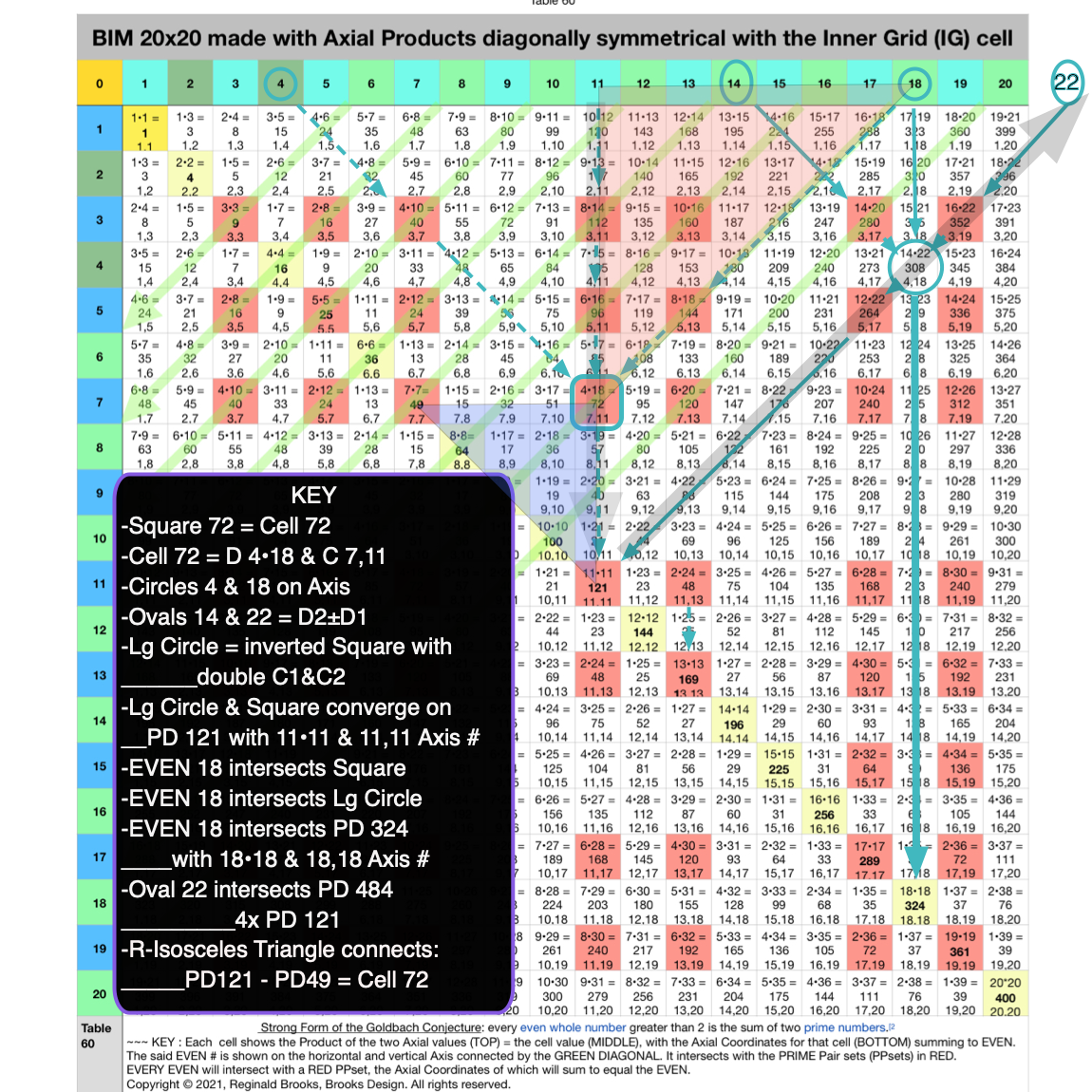Fig. 4.14 BIM-Goldbach_Conjecture, IV-14. Square 72 LINE, LAYOUT & SHAPE Cell pattern.

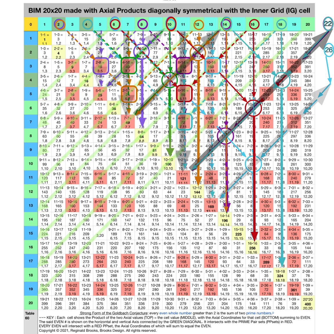Fig. 4.15 BIM-Goldbach_Conjecture, IV-15. Relating all 7 examples with their DIAGONAL pattern.

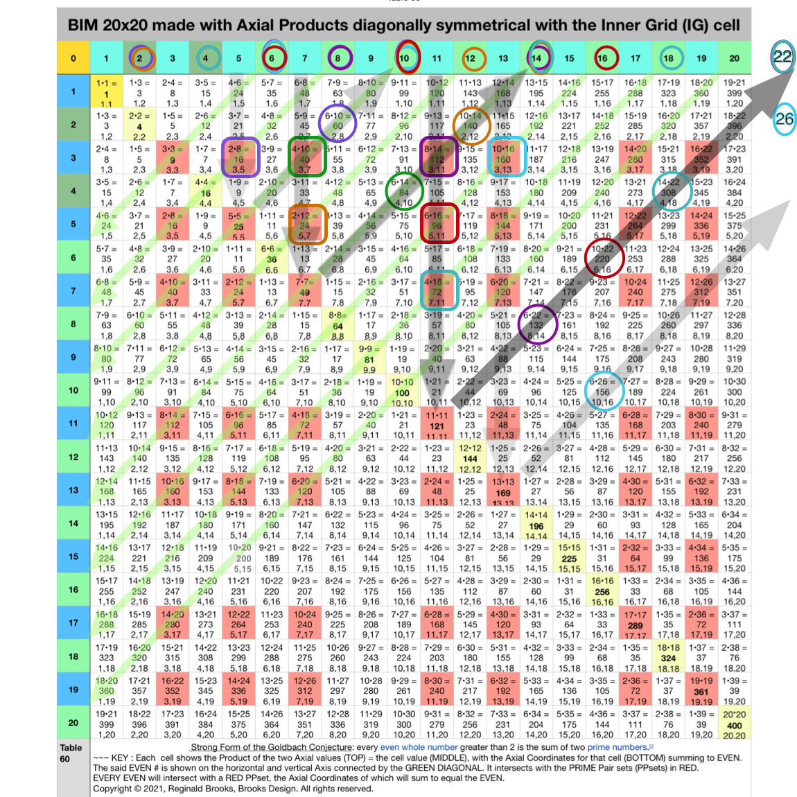Fig. 4.16 BIM-Goldbach_Conjecture, IV-16. Relating all 7 examples with their DIAGONAL pattern simplified.

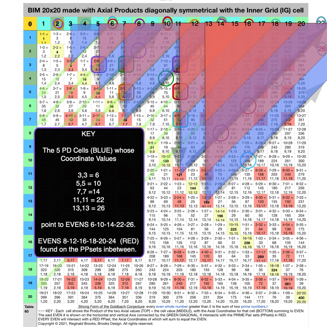Fig. 4.17 BIM-Goldbach_Conjecture, IV-17. Relating all 7 examples by SHAPE with their DIAGONAL pattern to their EVENS.

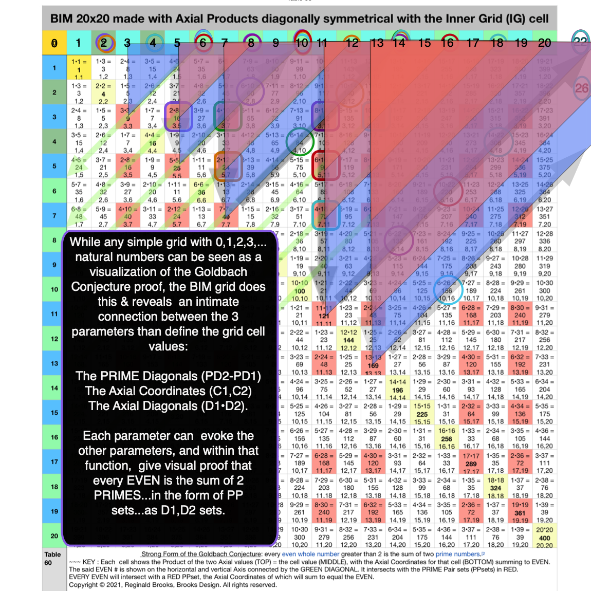Fig. 4.18 BIM-Goldbach_Conjecture, IV-18. Relating all 7 examples by SHAPE with their DIAGONAL pattern to their EVENS.

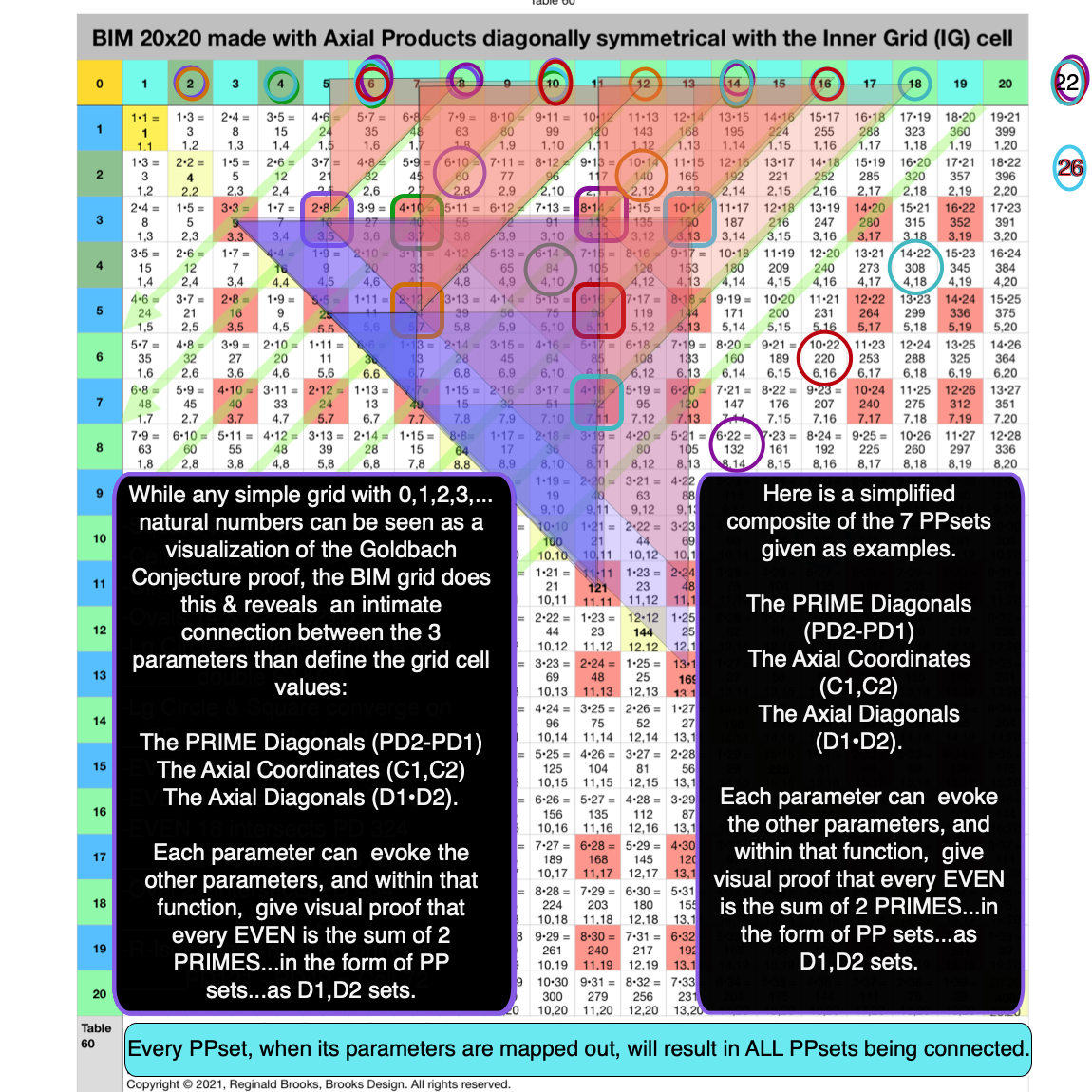Fig. 4.19 BIM-Goldbach_Conjecture, IV-19. Relating all 7 examples by SHAPE with their DIAGONAL & PD to their EVENS.

Using the R-Isosceles Triangle Shape is a very common practice in any examination of the BIM. It is no different here!

 

Summary

In Part IV, we shall combine Part I, II and III to see how each simple visualization step combines. In doing so, we will see that every PRIME Pair set (PPset) — i.e. those grid cells whose Axis Coordinate (C1, C2) are PPsets whose sum adds to said Axis EVEN # — when examined with all 3 parameters ultimately interconnects with every other PPset in defining the EVEN #s that they inform.

Not only can all 3 parameters presenting the difference in the intersecting PDs, the product of the Axial Diagonals and the sums of the Axial Coordinates, be readily visualized, but in addition the R-Isosceles Triangle Shape pops out naturally when visualizing how each "Parent" Cell relates to one or more of its "Child" Cells. These in turn relate back to the initial "Parent" PD values that itself points back to both the Cell and the EVEN number that its Axis Coordinates sum to. These can be seen as the connecting Diagonal. Plotting all such R-Isosceles Shapes reveals that each and every EVEN will have one or more intersecting Red Cells within its Axial Diagonal path.

While the details of the proof of Euler's Strong Form of the Goldbach Conjecture is specifically laid out in the Periodic Table Of PRIMES (PTOP) and PRIMES On the BIM (POP) works, the actual visualization could not be easier than right here on the BIM-Goldbach_Conjecture.

 

5. Conclusion

There are many reasons that the visualizations on the BIM is important, not the least of which is that:

• it shows an interconnectedness of all the PPsets that inform the EVENS;
• it contains the actual Periodic Table Of PRIMES (PTOP) that provides the working proof of Euler's Strong Form of the Goldbach Conjecture;
• it has some predictability for the "next" PPsets as well as a path back to all smaller PPsets;
• it contains within the matrix itself a definite separation -- and thus identity -- of ALL PRIMES from their non-PRIMES tag alongs;
• it fundamentally characterizes the symmetry and fractal-nature of the PPsets;
• it provides a definitive distribution of ALL possible PRIME positions as Active Rows --- the same Active Rows that the Primitive Pythagorean Triples occupy as possible PPTs.
• And it does all this within the ubiquitous and infinitely expandable BIM whose primary derivation and core functionality is in describing the Inverse Square Law (ISL)!

So it is within the BIM that we have now introduced further simple visualizations of how every EVEN ≥ 6 is the sum of two PRIMES.

 

REFERENCES

While there are no specific references for this work other than referring back to my own original work, there are many references involved in the study and research on the PRIMES in general. These have been well documented in the TPISC_IV: Details_BIM+PPT+PRIMES focus white paper. This paper also contains the background graphics and tables leading up to this current work. The focus page is part of the much larger TPISC_IV: Details ebook project that is freely available as an HTML webpage. The quick reference outline can be found here. An overall INDEX can be found here.

APPENDIX

Table 59. The flow of the Axis Diagonals Values on the BIM.

Table 60. The flow of the Axis Coordinates and Axis Diagonals Values on the BIM.

Table 61. The flow of the Axis Coordinates and Axis Diagonals Values on the BIM 20x20 is deconstructed to reveal its component parts.

In Table 61 the BIM 20x20 grid is deconstructed in to color coded parts. Each line presents info on the PRIME Pair set (PPset) whose members sum up to the respective EVEN #.

• line:  numbers 1,2,3,… for easy reference; (Light GRAY)
• Col #: Column number from the TOP horizontal Axis header of the BIM; (BLUE-GREEN)
• Row #: Row number from the Left SIDE vertical Axis header of the BIM: (Light BLUE)
• Cell Value: the number value of the BIM grid cell; (GREEN)
• C-Axis 1: First Coordinate Axis value (smallest first) of the two that intersect cell value; (BLUE-GREEN)
• C-Axis 2: Second Coordinate Axis value (smallest first) of the two that intersect cell value; (LightBlue)
• C Product: The Product of C1 • C2; (WHITE/GRAY)
• C Sum (∑): The Sum of C1 + C2; (RED)
• D-Axis 1: First DIAGONAL Axis value (smallest first) of the two that intersect cell value; (YELLOW)
• D-Axis 2: Second DIAGONAL Axis value (smallest first) of the two that intersect cell value; (PINK, and ORANGE for 
• 1/2 EVEN value)
• D Sum (∑): Sum of the two DIAGONAL Axis values; (BLUE)
• D Product: The Product of D1 • D2; (GREEN)

• C Product + D Sum (∑): Sum of the C Product + D Sum (∑); ( WHITE)

• ∆ C Product  & D Sum (∑): The difference of the C Product & D Sum (∑) values; ( WHITE/GRAY)

• EVEN #: The EVEN number that is the sum of the two PRIMES deconstructed on each line. (RED)

Note that the vertical COLOR columns specifically represent duplicate values. The dark GRAY columns separate the deconstruction into their component parts.

• First we have the Col, Row and actual Cell values for those specific cells on the BIM that are intersected by the diagonals running between two similar EVENS  (located on the Axis’).

• Second are the Coordinates (C). The Coordinates are the same as the Col & Row values. They are first multiplied together to give the C Product, and then separately added together to give the C Sum (∑) in RED.

• Third over are the D or Diagonal Axis values. Each BIM cell is composed of the product of two Axis values that diagonally converge on the Inner Grid cell. The only exception being the main Primary/Prime Diagonal (PD) cells that are the squares of the Axis values, respectively. Again, like the C-values above, the Diagonal values are added to give the D Sum (∑) (BLUE), and multiplied together to give the D Product in

• The Fourth segment examines the addition of the D Sum (∑) + C Product, giving the C Product + D Sum (∑) column of values in WGREEN. The D Product = Cell Value. The ORANGE D-Axis 2 values are found exclusively at cells on the PD. Their value is always 1/2 their respective EVEN value.HITE. This is followed by difference in the two values in WHITE or GRAY. 

• The Fifth, last segment, shows how the EVENS in RED are duplicated by the C Sum (∑) and D-Axis 2 values (also in Red). The latter values for the cell values landing on the PD are 1/2 the EVEN.

• The D1 value always gives the spread of the respective C1-C2 values (D1=C2-C1). D2 always gives the EVEN #, as does C1 + C2 (D2=C1+C2).

• The ∆ in the D1 & D2 values  + ∆ in the C1 & C2 values always adds up to give the EVEN # [EVEN=(D2-D1)+(C2-C1)].

• The D1 + C1 = C2 is always true except when the cell is on the PD (ORANGE) (C2=D2-C1 is also always valid with the same exception).

Study of the WHITE and WHITE/GRAY sections reveals intimate connections between the C—Coordinate  and the D-Diagonal Axial values informing the PRIME Pair sets shown. Of interest is how this deconstruction shows that any simple grid of natural whole integer numbers along the horizontal and vertical axis can reveal a simple and elegant visualization of  how every EVEN number is composed of the sum of two PRIMES. Combined with the Periodic Table Of PRIMES (PTOP) and PRIMES On the BIM  (POB), we have proof of Euler’s Strong Form of the GoldBach Conjecture!

SUMMARY

• C1•C2=CP
• C1+C2=C∑=EVEN
• C1+C2=*D2  ((
• D1+D2=D∑
• D1•D2=D1•(C1+C2)=DP=Cell Value
• D1=C2-C1
• D2=C1+C2
• C1=D2-C2
• C2=C1+*D1=D2-C1
• (D2-D1)+(C2-C1)=EVEN

NEW SUMMARY

◦C1,C2=Cell Location by Coordinates

◦C1+C2=EVEN

◦C1+C2=*D2  (*except PD)

◦C1=(D2-D1)/2

◦C1=D2-C2

◦C2=(D1+D2)/2

◦C2=C1+*D1=D2-C1

◦D1•D2=Cell Value by Axis Diagonals product

◦D1•D2=D1•(C1+C2)

◦D1=C2-C1

◦D2=C1+C2

◦(D2-D1)+(C2-C1)=EVEN