Part III

You know, it all started when I was trying to visualize how the

Inverse Square Law (ISL)

would play out on a simple grid of whole integer numbers.

 

That led to the BIM (BBS-ISL Matrix) grid discovery.

 

Here is Part III of the simplified BIM with some new takes!

 

The visual solution to the Goldbach Conjecture has never been simpler or more elegant!

 

Intro

 

Let's start where the main Part I and especially Part II finished:

 

~~ ~~ ~~ ~~ ~~ ~~ from Part I Summary ~~ ~~ ~~ ~~ ~~ ~~

Summary

As the PTOP has shown that the number of PPsets growth rate exceeds the PRIMES span rate, combined with the infinite distribution of the PPset within the infinite expansion of the BIM itself, we can say with confidence that:

 

Every EVEN # (≥2, or include 2 if you consider 1 to be prime, as the ancients did) is composed of one or more pair sets of PRIMES.

 

And in its most simplified restatement:

 

On the BIM, DIAGONALS between Axial EVENS intersect their composing PPsets.

 

 

~~ ~~ ~~ ~~ ~~ ~~ from Part II Summaries & Conclusion ~~ ~~ ~~ ~~ ~~ ~~

 

So it is within the BIM that we have now introduced further simple visualizations of how every EVEN ≥ 6 is the sum of two PRIMES.

Four short videos have been produced. Each reveals a simple visual concept that builds on that which it follows:

1. Lines:
2. Layout:
3. Shape:
4. Integration:

 

1. Lines

Summary

In perhaps the simplest visualization of the Goldbach Conjecture — Euler’s Strong Form of the Goldbach Conjecture states that every EVEN number is the sum of two PRIMES — on the BIM.

 

A Diagonal line connecting two similar EVENS from one Axis to the other will intersect the grid cells whose coordinate values sum up to said EVEN.

 

Nothing could be easier to visualize and as the BIM (BBS-ISL Matrix) expands to infinity, so does the solution to the Goldbach Conjecture. Note: it has been shown that the conjecture is valid up to EVENS 10^18.

 

This work follows on the heels of the Periodic Table Of the PRIMES (PTOP) and PRIMES On the BIM (POB) earlier this year (2020). These works provide the details of the inherent fractal nature of the PRIMES when treated as PRIME Pair sets (PPsets). The fractal disposition results in a strictly symmetrical distribution of the PPsets about ANY and ALL possible EVENS. And they do so at a rate that exceeds the rate of the PRIME Gaps ensuring that NO EVEN is devoid of at least one PPset whose members sum to that EVEN.

 

 

2. Layout

Summary

In Part II, we have had a further simplification! Though at first glance it may seem more complicated, it really is not once you realize that every cell in the BIM follows this same pattern. Each grid cell is defined by two sets of Axis numbers:

 

1. The Axis Coordinates (C1 & C2)— one on the Top horizontal Axis and one on the Left vertical Axis — provide the grid cell LOCATION. They are found on the BOTTOM of the Cell grid;
2. The Axis Diagonals (D1 & D2)— both values from either the Top horizontal or the Left-side vertical Axis — diagonally converge on a grid cell VALUE. They are found on the TOP of the Cell grid.

 

Together, these two sets of values provide information about that respective grid cell value, inter-relate to each other, and inform — when in Diagonal line — the value of the related EVEN number they are connected with!

 

Here is a SUMMARY:

 

◦C1,C2=Cell Location by Coordinates

◦C1+C2=EVEN

◦C1+C2=D2 (except PD)

◦C1=(D2-D1)/2

◦C1=D2-C2

◦C2=(D1+D2)/2

◦C2=C1+*D1=D2-C1

◦D1•D2=Cell Value by Axis Diagonals product

◦D1•D2=D1•(C1+C2)

◦D1=C2-C1

◦D2=C1+C2

◦(D2-D1)+(C2-C1)=EVEN

 

 

3. Shape

Summary

In Part III, we have had a further simplification: Right-Isosceles Triangles!

 

In Part II we wrote: Though at first glance it may seem more complicated, it really is not once you realize that every cell in the BIM follows this same pattern. Each grid cell is defined by two sets of Axis numbers:

 

1. The Axis Coordinates (C1 & C2)— one on the Top horizontal Axis and one on the Left vertical Axis — provide the grid cell LOCATION;

2. The Axis Diagonals (D1 & D2)— both values from either the Top horizontal or the Left-side vertical Axis — diagonally converge on a grid cell VALUE.

   Actually, if one considers just the Inner Grid (IG) cells, a third parameter:

3. The difference in the Prime Diagonals (PD2 - PD1) — from the Row & Column intersect — provide the grid cell VALUE, too.

 

All 3 of the above parameters can be represented by a Right-angled Isosceles Triangle.

 

Part III presents examples of a number of grid cells that intersect with the Axis EVEN #s via a Diagonal between the two Axis’. We do so with the 3 parameters defining said grid cell defined by their 3 colored R-Isosceles Triangles.

 

 

4. Integration

Summary

In Part IV, we shall combine Part I, II and III to see how each simple visualization step combines. In doing so, we will see that every PRIME Pair set (PPset) — i.e. those grid cells whose Axis Coordinate (C1, C2) are PPsets whose sum adds to said Axis EVEN # — when examined with all 3 parameters ultimately interconnects with every other PPset in defining the EVEN #s that they inform.

Not only can all 3 parameters presenting the difference in the intersecting PDs, the product of the Axial Diagonals and the sums of the Axial Coordinates, be readily visualized, but in addition the R-Isosceles Triangle Shape pops out naturally when visualizing how each "Parent" Cell relates to one or more of its "Child" Cells. These in turn relate back to the initial "Parent" PD values that itself points back to both the Cell and the EVEN number that its Axis Coordinates sum to. These can be seen as the connecting Diagonal. Plotting all such R-Isosceles Shapes reveals that each and every EVEN will have one or more intersecting Red Cells within its Axial Diagonal path.

While the details of the proof of Euler's Strong Form of the Goldbach Conjecture is specifically laid out in the Periodic Table Of PRIMES (PTOP) and PRIMES On the BIM (POP) works, the actual visualization could not be easier than right here on the BIM-Goldbach_Conjecture, II.

 

5. Conclusion

There are many reasons that the visualizations on the BIM is important, not the least of which is that:

• it shows an interconnectedness of all the PPsets that inform the EVENS;


• it contains the actual Periodic Table Of PRIMES (PTOP) that provides the working proof of Euler's Strong Form of the Goldbach Conjecture;


• it has some predictability for the "next" PPsets as well as a path back to all smaller PPsets;


• it contains within the matrix itself a definite separation -- and thus identity -- of ALL PRIMES from their non-PRIMES tag alongs;


• it fundamentally characterizes the symmetry and fractal-nature of the PPsets;


• it provides a definitive distribution of ALL possible PRIME positions as Active Rows --- the same Active Rows that the Primitive Pythagorean Triples occupy as possible PPTs.


• And it does all this within the ubiquitous and infinitely expandable BIM whose primary derivation and core functionality is in describing the Inverse Square Law (ISL)!

So it is within the BIM that we have now introduced further simple visualizations of how every EVEN ≥ 6 is the sum of two PRIMES.

Four short videos have been produced. Each reveals a simple visual concept that builds on that which it follows:

1. Lines:
2. Layout:
3. Shape:
4. Integration:

 

~~ ~~ ~~ ~~ ~~ ~~ end of Part I & Part II Summaries and Conclusion ~~ ~~ ~~ ~~ ~~ ~~

 

Part III of the BIM-Goldbach Conjecture

In Part III we will be showing how simply switching around the Axis Coordinates and Axis Diagonals from Parts I and II gives us the Periodic Table Of PRIMES (PTOP). That's right! Simply moving the Axis Coordinate values to the Cell TOP reproduces the original PTOP.

To make the visualization both simpler and in the same format as the original PTOP we will first show this transformation on the LOWER half of the BIM, but then move it back to the UPPER BIM presentation.

What does this accomplish?

What we are really doing is looking at the same relationships between the numbers on the BIM grid. The switching of the Axis Coordinate and Diagonal Cell ID positions is like seeing the same information from a different perspective afforded by looking at it through a different lens.

Here is the key: In the standard, base BIM view of BIM-Goldbach_Conjecture Part I and II, we see a DIRECT relationship between the LINES (Diagonal), LAYOUT (Axis D on TOP, Axis C on BOTTOM of each Cell), SHAPE (R-Triangle) and INTEGRATION (All interconnect) of the grid with the EVENS; while in this NEW BIM-Goldbach_Conjecture, Part III version we see a more INDIRECT visualization of the same grid with the EVENS. In the latter, we are seeing the derivation of the PTOP with greater emphasis on the PRIME Pair sets (PPsets) as the symmetry dependent, fractal that informs each an every EVEN. It does do by splaying out the PPset about 1/2 half the EVEN value -- a process that both expands the grid needed to see each EVEN and provides the basis for the proof in satisfying the Goldbach Conjecture! It was covered in full detail in the Periodic Table Of PRIMES (PTOP) and PRIMES On the BIM (POB) works. Once again, the R-Triangle, especially a large R-Isosceles Triangle can be rotated from any given Cell value to generate ALL the values throughout the BIM grid!

And while this NEW-revert to the original PTOP version adds complexity, it really is not all that much more.

The Coordinate values simply give you location data: From what position on the horizontal and vertical Axis does this Cell occupy.

The Diagonal values gives the Cell value, but it does so as the two Axis multiplier values.

The difference then, in this key takeaway, is that if you look at the Diagonal values in the DIRECT perspective view, you get the simple straightforward visualizatiion of those Diagonal lines coming from each Axis EVEN intersecting the grid Cells whose Coordinate values sum up to said EVENS.

If instead, you flip your lens to see those PPsets that made up the Coordinates in the DIRECT view are now switched up to become the NEW Coordinates for each Cell to give the INDIRECT view. The INDIRECT view splays open the DIRECT view so that the actual Axis EVENS are symmetrically divided in half. In doing so, we are now lead to look at the EVEN/2 and see directly how the PPsets that inform those EVENS lie symmetrical to either side.

Along the way, we see how Diagonals back from these PPsets to the central dividing line vertex as 90° Right Isosceles Triangles.

The STEPS counted along the way match the separations between the PPset members and the EVEN/2 values.

Because more than one PPset is usually involved in informing its EVEN, we readily see these as symmetrical, fractal units that when tabulated onto the PTOP reveals exactly how these overlapping PPsets grow at a pace that far exceeds that of the gaps between the PRIMES, thus ensuring that every EVEN has one or more PPsets that sum to its value.

This PTOP grows rapidly and extends to infinity, as does the BIM from that which it was derived! I invite you, dear reader, to review the earlier, more detailed work on the PTOP to see how this very intriguing fractal of PPsets are formed.

It is within that context -- that by seeing how all the pieces work and rotate together that the bigger picture actually does simplify!

 

IMAGES: Part III of the BIM-Goldbach Conjecture

 



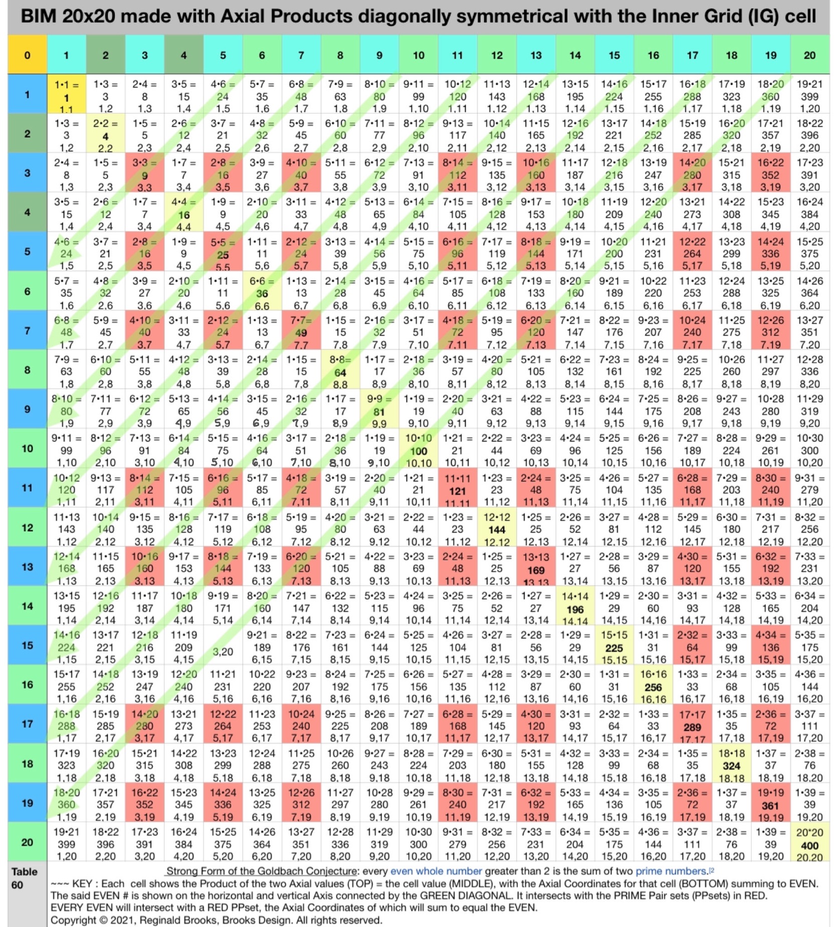
Fig.1. The DIRECT view of the EVENS Diagonals intersecting the Cells whose Axis Coordinates (at the BOTTOM of each RED Cell) sum up to their respective EVENS.

 

 

 



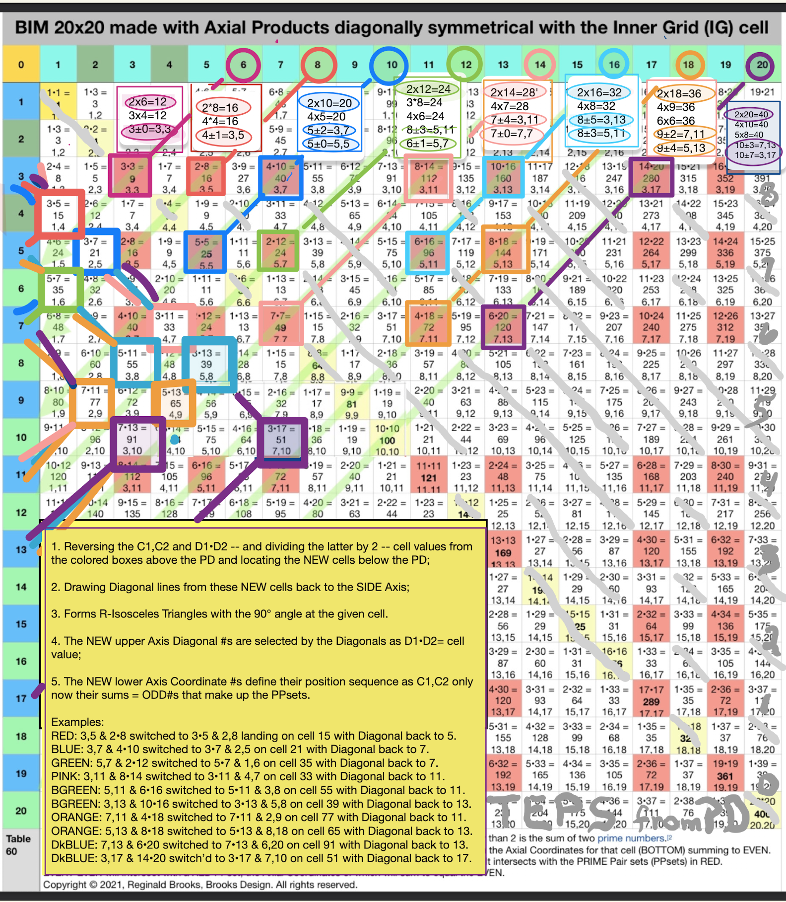
Fig.2. Switching the Axis Coordinates (C1,C2) found in th UPPER BIM to Axis Diagonals in the LOWER BIM, effectively reveals the Periodic Table Of PRIMES (PTOP).

For example, the Cell 280 with C1=3 and C2=17 in the UPPER BIM is switched to D1=3 and D2=17 Axis Diagonals in the LOWER BIM at Cell 51.

Notice in doing so, that the NEW LOWER Axis Coordinates are 1/2 the UPPER value.

Now at LOWER Cell 51, path straight back to Axis=10. 10 x 2 = 20 and this path intersects the 1st Parallel Diagonal at Cell 19 that is raised to 20 when exploring the PTOP, only here everything is on the LOWER BIM.

ALL Axis Coordinates here in the LOWER BIM sum up to PRIMES as they are part o the PPset that make up said EVEN 20!

 



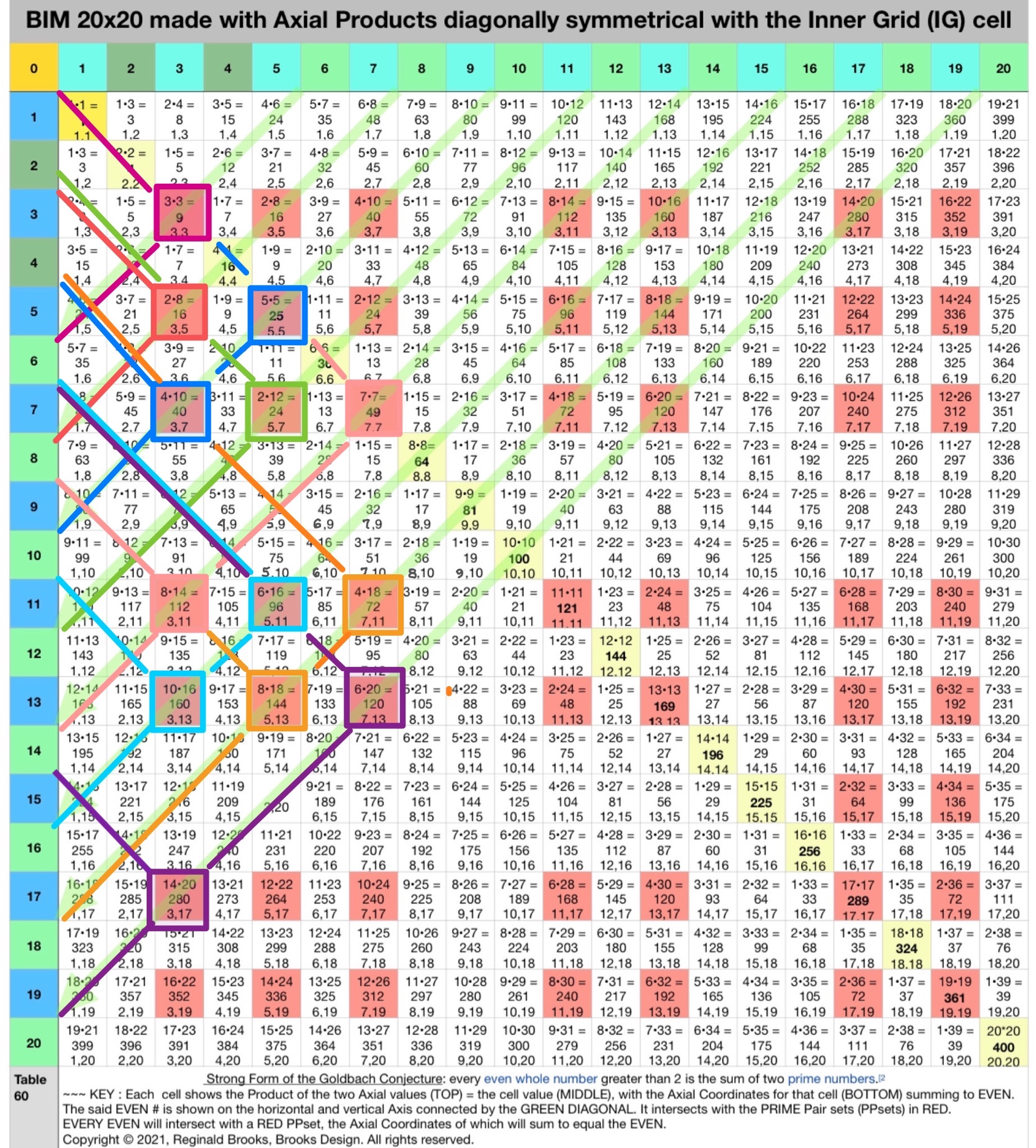
Fig.3. Here it cleaned up. Now, to be consistent with the earlier PTOP, let's move the examples in the LOWER BIM back up to the UPPER BIM while switching the PPsets now to the TOP of the individual Cells (circled). See the next figure.

 

 

 



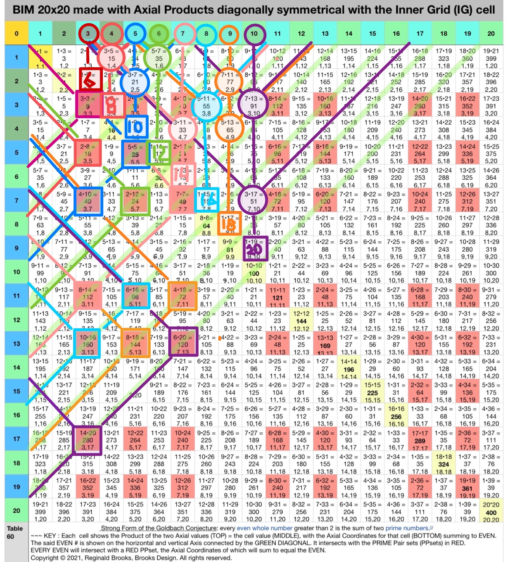
Fig.4. The Circled values on the TOP horizontal Axis all individually reference as being the EVEN/2, i.e. that value x 2 is the EVEN under consideration.

The EVEN/2 value is the centerline path back down to "altered" 1st Parallel Diagonal, just prior to landing on the PRIME Diagonal (PD).

The Light GREEN Diagonals from the PD point back up to the respective EVEN on the TOP horizontal Axis.

The STEPS from the EVEN/2 down the straight path to the PD reflect the symmetrically separated PPset values to either side of said EVENS. These PPset values are on the TOP of the Cell and reflect the Axis Diagonal values, i.e. their product equals the Cell value.

 

 

 



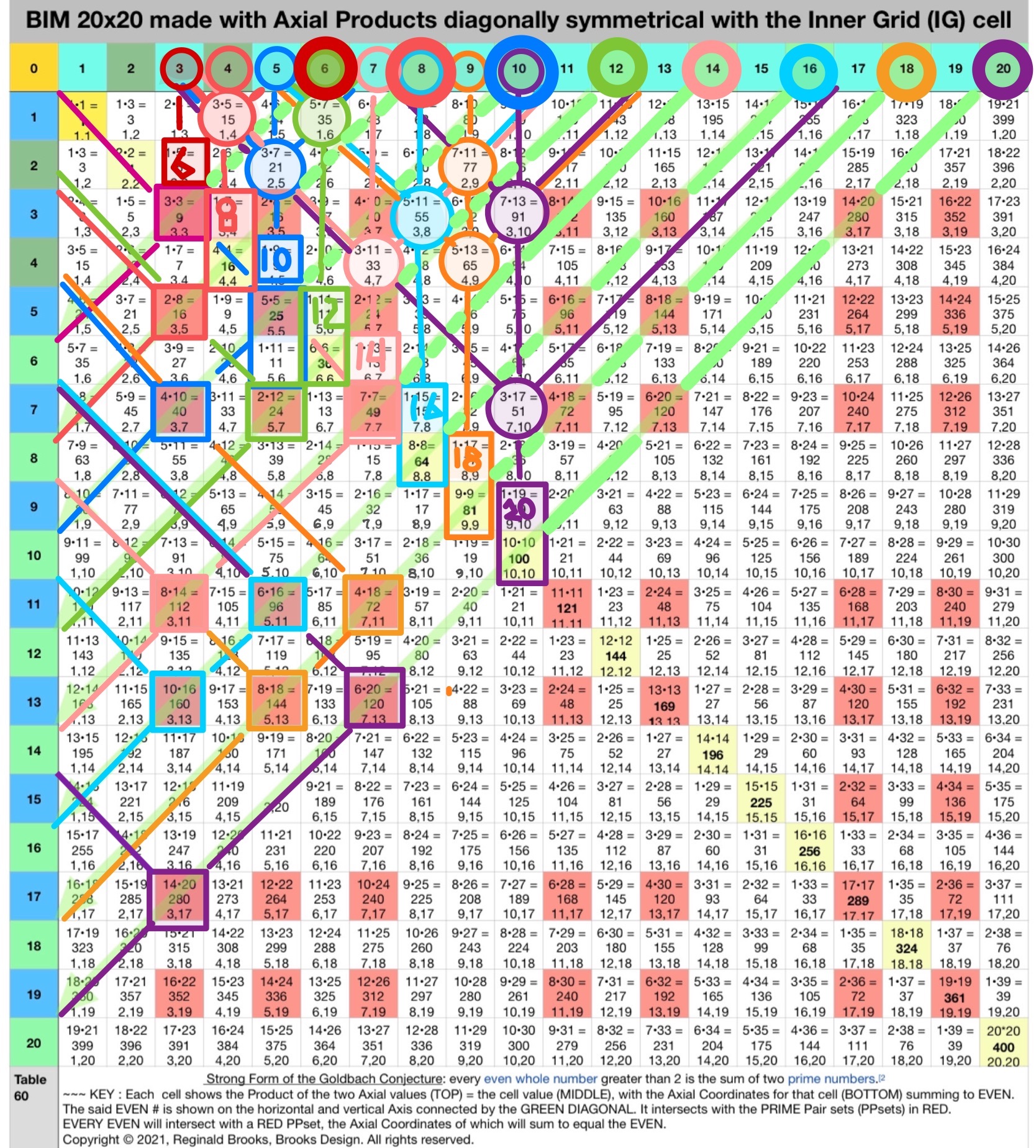
Fig.5. To complete the graphic, the actual full EVENS on the TOP horizontal Axis are given a large, thick Circle. They, of course, represent the doubling of the EVEN/2 smaller Axis Circles. Additionally, the Squares of the Cells on the 1st Parallel Diagonal have been enlarged to Rectangles enclosing the PD Cell as well.

The persistent, ubiquitous and infinitely expanding symmetry of the PRIMES as PPsets book shelving each EVEN/2 is fundamental to understanding how the PRIMES -- as the atomic numbers -- form ALL the EVENS in combo pair sets of two, and, do so in a fractal manner.

That fractal manner is simply the overlapping of the same identical PRIMES Sequence onto successive PRIME Sequences, generating along the way, the PTOP phennomen that elucidates this beautiful pattern! It is really only apparent on the PTOP (see image towards bottom of this page).

The non-prime ODDS -- *being composed of three PRIMES -- can be said to exist out of default, if you will. They are simply redundant in the sense that they are both composite numbers and are not needed, per se, to form the EVENS or, for that fact, any other ODD -- any other number, really -- as the PRIMES can do it all!

 

*In number theory, Goldbach's weak conjecture, also known as the odd Goldbach conjecture, the ternary Goldbach problem, or the 3-primes problem, states that

Every odd number greater than 5 can be expressed as the sum of three primes. (A prime may be used more than once in the same sum.)

This conjecture is called "weak" because if Goldbach's strong conjecture (concerning sums of two primes) is proven, then this would also be true. For if every even number greater than 4 is the sum of two odd primes, adding 3 to each even number greater than 4 will produce the odd numbers greater than 7 (and 7 itself is equal to 2+2+3).

In 2013, Harald Helfgott published a proof of Goldbach's weak conjecture.[2] As of 2018, the proof is widely accepted in the mathematics community,[3] but it has not yet been published in a peer-reviewed journal.

(https://en.wikipedia.org/wiki/Goldbach%27s_weak_conjecture)

 

For clarity, let's repeat:

Here is the key: In the standard, base BIM view of BIM-Goldbach_Conjecture Part I and II, we see a DIRECT relationship between the LINES (Diagonal), LAYOUT (Axis D on TOP, Axis C on BOTTOM of each Cell), SHAPE (R-Triangle) and INTEGRATION (All interconnect) of the grid with the EVENS; while in this NEW BIM-Goldbach_Conjecture, Part III version we see a more INDIRECT visualization of the same grid with the EVENS. In the latter, we are seeing the derivation of the PTOP with greater emphasis on the PRIME Pair sets (PPsets) as the symmetry dependent, fractal that informs each an every EVEN. It does do by splaying out the PPset about 1/2 half the EVEN value -- a process that both expands the grid needed to see each EVEN and provides the basis for the proof in satisfying the Goldbach Conjecture! It was covered in full detail in the Periodic Table Of PRIMES (PTOP) and PRIMES On the BIM (POB) works. Once again, the R-Triangle, especially a large R-Isosceles Triangle can be rotated from any given Cell value to generate ALL the values throughout the BIM grid!

And while this NEW-revert to the original PTOP version adds complexity, it really is not all that much more.

The Coordinate values simply give you location data: From what position on the horizontal and vertical Axis does this Cell occupy.

The Diagonal values gives the Cell value, but it does so as the two Axis multiplier values.

The difference then, in this key takeaway, is that if you look at the Diagonal values in the DIRECT perspective view, you get the simple straightforward visualizatiion of those Diagonal lines coming from each Axis EVEN intersecting the grid Cells whose Coordinate values sum up to said EVENS.

If instead, you flip your lens to see those PPsets that made up the Coordinates in the DIRECT view are now switched up to become the NEW Coordinates for each Cell to give the INDIRECT view. The INDIRECT view splays open the DIRECT view so that the actual Axis EVENS are symmetrically divided in half. In doing so, we are now lead to look at the EVEN/2 and see directly how the PPsets that infrom those EVENS lie symmetrical to either side.

Along the way, we see how Diagonals back from these PPsets to the central dividing line vertex as 90° Right Isosceles Triangles.

The STEPS counted along the way match the separations between the PPset members and the EVEN/2 values.

Because more than one PPset is usually involved in informing its EVEN, we readily see these as symmetrical, fractal units that when tabulated onto the PTOP reveals exactly how these overlapping PPsets grow at a pace that far exceeds that of the gaps between the PRIMES, thus ensuring that every EVEN has one or more PPsets that sum to its value.

This PTOP grows rapidly and extends to infinity, as does the BIM from that which it was derived! I invite you, dear reader, to review the earlier, more detailed work on the PTOP to see how this very intriguing fractal of PPsets are formed.

It is within that context -- that by seeing how all the pieces work and rotate together that the bigger picture actually does simplify!

 

 

Here is a short video overview:

PTOP: Periodic Table Of PRIMES & the Proof of the Goldbach Conjecture

BIM-Goldbach_Conjecture_IV from Reginald Brooks on Vimeo.

PTOP Goldbach Conjecture from Reginald Brooks on Vimeo.

 



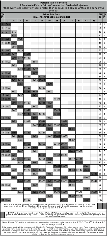
Fig.6. The original PTOP from 2009... more here at Brooks (Base) Square and the Inverse Square Law (ISL).

 

Easy reference to all the PRIMES White Papers: PRIMES INDEX

 

Graphic Layout to all Math-Art-Physics works

 

BIM-Goldbach_Conjecture: Part I and II

 

 

 

~~ ~~ ~~ ~~ ~~ ~~ SPECULATION ~~ ~~ ~~ ~~ ~~ ~~

Force of Numbers (FON)

The Force Of Numbers (FON), or Numbers Force, is proposed to be that by which a Pattern In Number (PIN) becomes the favored path, i.e. a force, that generates an expression, a.k.a. pattern.

In Newtonian physics, we think of force (F) as mass (m) times acceleration (a) as F=ma.

(wikipedia: https://en.wikipedia.org/wiki/Force)

In the Standard Model of Quantum Mechanics we describe the four (4) fundamental interactions or forces of Nature:

1. Gravitational

2. Electromagnetic

3. Weak nuclear

4. Strong nuclear

(5.) speculative.

In physics, the fundamental interactions, also known as fundamental forces, are the interactions that do not appear to be reducible to more basic interactions. There are four fundamental interactions known to exist: the gravitational and electromagnetic interactions, which produce significant long-range forces whose effects can be seen directly in everyday life, and the strong and weak interactions, which produce forces at minuscule, subatomic distances and govern nuclear interactions. Some scientists hypothesize that a fifth force might exist, but these hypotheses remain speculative.[1][2][3] (wikipedia: https://en.wikipedia.org/wiki/ Fundamental_interaction)

But what about the FON? First, let’s define “number.”

A number is a mathematical object used to count, measure, and label. The original examples are the natural numbers 1, 2, 3, 4, and so forth.[1] Numbers can be represented in language with number words. More universally, individual numbers can be represented by symbols, called numerals; for example, "5" is a numeral that represents the number five. As only a relatively small number of symbols can be memorized, basic numerals are commonly organized in a numeral system, which is an organized way to represent any number. The most common numeral system is the Hindu–Arabic numeral system, which allows for the representation of any number using a combination of ten fundamental numeric symbols, called digits.[2][3] In addition to their use in counting and measuring, numerals are often used for labels (as with telephone numbers), for ordering (as with serial numbers), and for codes (as with ISBNs). In common usage, a numeral is not clearly distinguished from the number that it represents.

In mathematics, the notion of a number has been extended over the centuries to include 0, [4] negative numbers,[5] rational numbers such as one half (1/2), real numbers such as the square root of 2 (√2) and π,[6] and complex numbers[7] which extend the real numbers with a square root of −1 (and its combinations with real numbers by adding or subtracting its multiples).[5] Calculations with numbers are done with arithmetical operations, the most familiar being addition, subtraction, multiplication, division, and exponentiation. Their study or usage is called arithmetic, a term which may also refer to number theory, the study of the properties of numbers. (Wikipedia: https://en.wikipedia.org/wiki/Number)

One last quote: Feynman Diagrams and Paths:

In theoretical physics, a Feynman diagram is a pictorial representation of the mathematical expressions describing the behavior and interaction of subatomic particles. The scheme is named after American physicist Richard Feynman, who introduced the diagrams in 1948. The interaction of subatomic particles can be complex and difficult to understand; Feynman diagrams give a simple visualization of what would otherwise be an arcane and abstract formula. ....

Particle-path interpretation[edit] A Feynman diagram is a representation of quantum field theory processes in terms of particle interactions. The particles are represented by the lines of the diagram, which can be squiggly or straight, with an arrow or without, depending on the type of particle. A point where lines connect to other lines is a vertex, and this is where the particles meet and interact: by emitting or absorbing new particles, deflecting one another, or changing type.

There are three different types of lines: internal lines connect two vertices, incoming lines extend from "the past" to a vertex and represent an initial state, and outgoing lines extend from a vertex to "the future" and represent the final state (the latter two are also known as external lines). Traditionally, the bottom of the diagram is the past and the top the future; other times, the past is to the left and the future to the right. When calculating correlation functions instead of scattering amplitudes, there is no past and future and all the lines are internal. The particles then begin and end on little x's, which represent the positions of the operators whose correlation is being calculated.

Feynman diagrams are a pictorial representation of a contribution to the total amplitude for a process that can happen in several different ways. When a group of incoming particles are to scatter off each other, the process can be thought of as one where the particles travel over all possible paths, including paths that go backward in time. (https://en.wikipedia.org/wiki/ Feynman_diagram)

 

So let’s put this together and see how there may be force operating below.

1. Fundamental Forces/Interactions result from the exchange of “force carrier particles;”

2. A pathway — path — establishes the connection;

3. While all possible paths must be considered, a statistically favored path becomes manifest upon reaching the final state;

Of all the multi-potential, multi-possible paths, a “favored” path statistically becomes operative. Why?

Perhaps, and what is being proposed here, is the who, what, where, when, how and why mechanism underlying that “favored” path is none other than numbers — quantifying natural whole integer numbers — and the patterns that their interconnections make.

What patterns?

The Inverse Square Law (ISL) is central to any formulation of spacetime.

Inverse-square law:

(From Wikipedia, the free encyclopedia)

In science, an inverse-square law is any scientific law stating that a specified physical quantity is inversely proportional to the square of the distance from the source of that physical quantity. The fundamental cause for this can be understood as geometric dilution corresponding to point-source radiation into three-dimensional space.(https://en.wikipedia.org/wiki/Inverse-square_law)

 

 

How do we get a pattern out of the ISL?

In 2009, in an attempt to formulate a grid pattern of the ISL, a discovery was made. It was called the Brooks (Base) Square - Inverse Square Law Matrix, later to be referenced as the BBS-ISL Matrix, and abbreviated again to its current acronym, BIM.

Brooks (Base) Square - Inverse Square Law Matrix = BBS-ISL Matrix = BIM

The BIM is a ubiquitous, infinitely expandable and powerful Pattern In Numbers (PIN) based solely on natural whole integer numbers, 0,1,2,3,...

Besides the literally hundreds of patterns within the BIM grid, are a few that really stand out as pivotal.

1. Every Pythagorean Triple — both Primitive “parent” and all the non- Primitive “child” — is present and interconnected on the BIM;

2. Every PRIME — present in an otherwise stealthily fashion — is completely present as symmetrical, fractal-like PRIME Pair sets (PPsets) that inform every possible EVEN number, and, along with forming the Periodic Table Of PRIMES (PTOP), give proof to Euler’s Strong Form of the Goldbach Conjecture: every EVEN is the sum of two PRIMES;

3. The Exponentials of all numbers are fully present as a pattern on the BIM.

Each of the three exceptional PINS above represent distinct patterns — or paths! — that are different from the pure square-pure circle patterns of the parent BIM. These PINS go in a different direction!

 

Squares become non-square rectangles, circles become ovals, lines become areas, and areas become volumes,...

If a force is a “favored” path, then a “favored” pattern must be considered the same — a “favored” path.

If you are a spacetime forming and you emanate from a singularity — perhaps easily represented here as zero — and upon your perfect circle-isosceles-square emanation you come across periodic nodes, nodes that now suggest a new “favored” non-circle, non-isosceles triangle, non-square path, you just may be statistically inclined, certainly upon the context of your emanation, to preferentially select one of these “favored” paths. In doing so, you have now started erecting a different — and perhaps richer — architectural scaffolding upon which subsequent spacetime emanations might be “favored” to follow. The expression of this “favored” path is very much a force in the construction of spacetime. The spacetime that contains the energy and interactions that we study as the Standard Model.

The Force Of Numbers or Numbers Force is the underlying pattern- driven force that informs the very formation and subsequent expression of any and all spacetime. It is the anti-entropic, fundamental organization of spacetime into a rich tapestry of interconnecting spacetime fields, expressed as particles and their interactions. Entropy itself may be defined as the “favored” path dissolution back to that of the core base ISL from which it emanated.

Entropy predicts that certain processes are irreversible or impossible, aside from the requirement of not violating the conservation of energy, the latter being expressed in the first law of thermodynamics. Entropy is central to the second law of thermodynamics, which states that the entropy of isolated systems left to spontaneous evolution cannot decrease with time, as they always arrive at a state of thermodynamic equilibrium, where the entropy is highest. (https://en.wikipedia.org/wiki/Entropy)

 

May the Force Of Numbers be with you!